The life-cycle hypothesis was postulated by Ando and Modigliani in an attempt to explain the behaviour of consumption function in the long and short run. According to this theory, current consumption decisions are based on future expected income over an individual’s lifetime. The major advantage of this theory is that Ando and Modigliani incorporated the role of assets in determining consumption decisions. Other theories don’t incorporate assets into consumption (absolute income hypothesis) or the role of assets is only implicit (permanent income hypothesis).
Econometrics Tutorials with Certificates
MPC < APC in cross-sections
Over the lifetime of any individual, income is low in the early years of life. As people reach middle age, their income rises as they start earning more. In later years of life, however, income starts falling again to reach low levels owing to retirement or the inability to work as people grow older. Therefore, income starts from a low level, keeps increasing in middle age, and declines back to a low level in old age.
In the case of consumption, individuals are expected to maintain a constant or slightly increasing level of consumption as they keep growing older. Since consumption is dependent on future expected income, the present value of consumption is constrained by the present value of income.
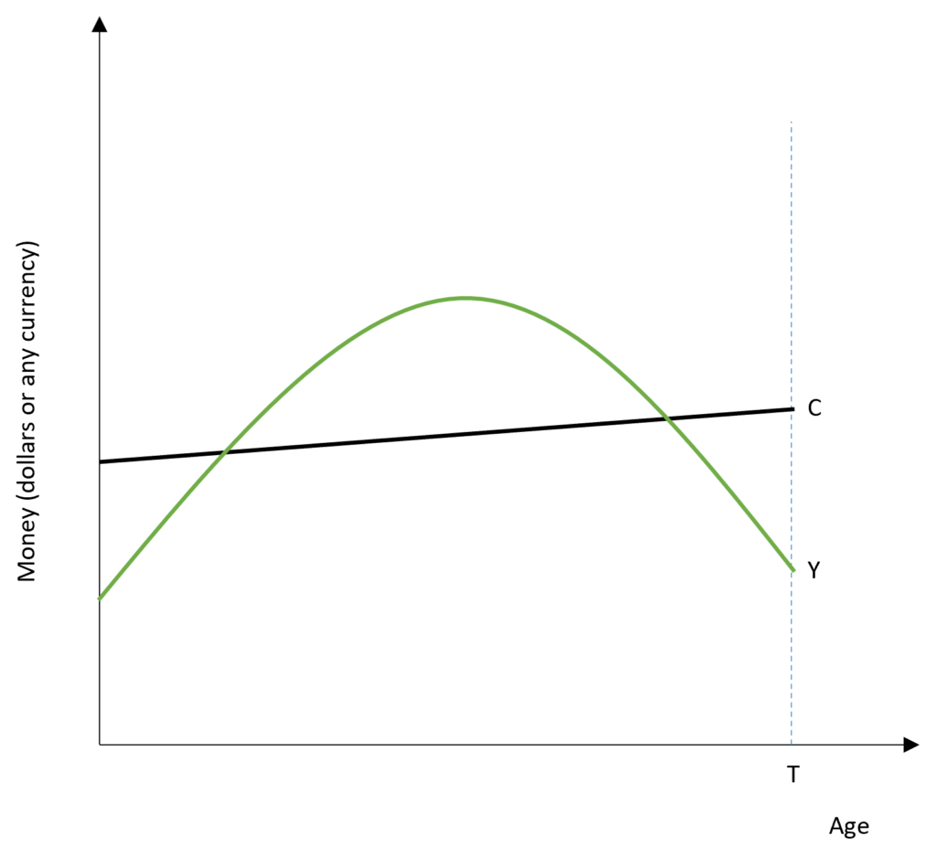
APC and MPS at different age
During the early years, income is low as compared to consumption and individuals are borrowers during this period, i.e. APC is high. However, they expect their future income to rise during their middle age. Because income is higher than consumption level, they pay off their borrowings during this period and save for retirement in old age. With high income, APC is low because consumption is much lower as compared to income in this period. In the later years of the life-cycle, income is again below consumption level. Hence, this is a period of dissavings or negative savings by individuals, leading to a low APC.
Therefore, across different sections based on income levels, APC will be high for low-income groups. These low-income groups primarily include people in their early years of life and people in old age, who have low incomes. On average, APC will be high as the low-income group consists of higher than average young and older people. On the contrary, high-income groups will have a higher than average proportion of middle-aged people. This is because they have higher incomes. APC, in this case, will be lower because consumption is low compared to income level during middle age.
Hence, APC will decline as income increases and MPC<APC in cross sections because of different income levels in a life-cycle.
consumption function of Life-Cycle Hypothesis
According to the life-cycle hypothesis, the consumption of any individual is based on expected income in the future. If the expected income rises, the consumption of that consumer will also increase. Ando and Modigliani use the Present Value criterion to represent expected income in the future. Therefore, the consumption of an individual can be expressed as follows:

If the present value of expected income increases, then consumption of that consumer will increase by a given proportion (theta) of that increase in income.
If the income distribution and age of the population are stable along with the constant taste and preferences of consumers, then the aggregate consumption function can simply be obtained by summation of all individual consumption functions.

Present Value of expected future income
Future income is unknown and cannot be measured directly. Therefore, the present value of expected income has to be estimated indirectly. Ando and Modigliani divided income into two types- income labour and income from assets, and estimated the present value variable as follows:
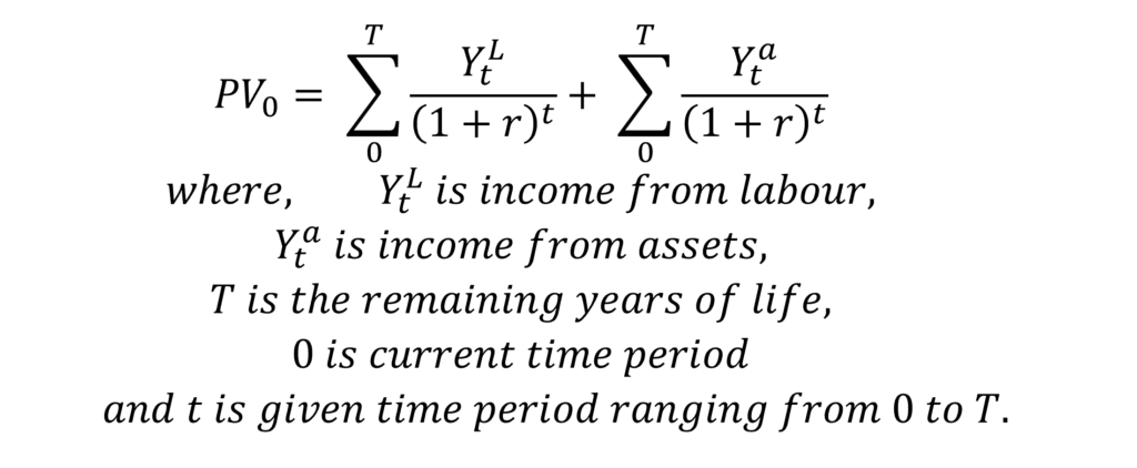
In an efficient capital market, we can assume that the present value of income from assets is equal to the value of assets in the current time period. Therefore, we can substitute the second element of the equation as:

In the case of the first element of income from labour, we know the labour income in the current period and can therefore separate current income from the present value of expected income.
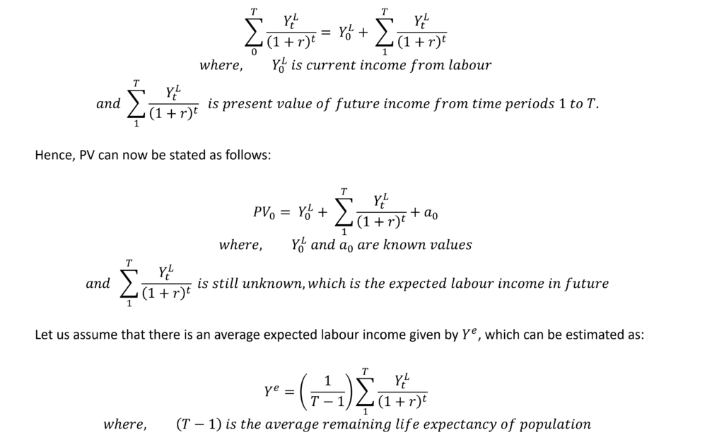
Therefore, the above equation simply divides the expected future labour income by the average life remaining of the population in years to estimate an average expected labour income. From this equation, we have:

In this equation, Ye is the only unknown which is an estimate of average expected labour income.
Ando and Modigliani found that assuming this average expected labour income as a function of current labour income worked well and they stated this as:

This implies that if current income increases, people expect average future income to rise as well. The amount of this rise is determined by the proportion coefficient (beta), such that an increase in average expected income is a proportion of current labour income.
Hence, we can modify the PV0 equation and the consumption function as follows:
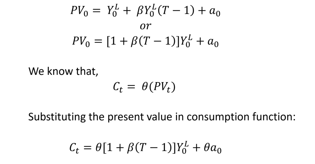
This equation represents the consumption function associated with the life-cycle hypothesis. Every variable in this equation can be measured which allows empirical estimation of the consumption function.
cyclical fluctuation and long-run consumption: empirical results
The consumption function put forward by Ando and Modigliani can be used to carry out empirical analysis to understand the behaviour of consumption in the long run and the effect of business cycles on consumption.
Ando and Modigliani applied this consumption function to annual data of the United States. They obtained the following results:

The marginal propensity to consume from labour income is 0.7. This means that a $1 increase in labour income will lead to a $0.7 increase in consumption. Similarly, the marginal propensity to consume from assets is 0.06 implying that a $1 increase in assets (net worth of assets) will lead to a $0.06 increase in consumption.
Let us apply these results to the life cycle consumption function:
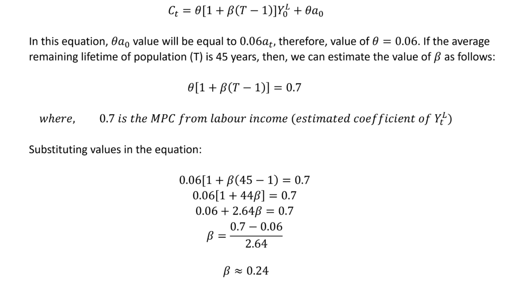
Hence, the positive coefficient beta suggests that with an increase in current labour income, the average expected labour income increases. As current labour income increases by $1, the average expected labour income increases by $0.25.
MPC and APC
This estimated consumption function has a slope of 0.7 or MPC, corresponding to the coefficient of YtL. The intercept of the consumption function is equal to 0.06at because assets remain the same in the short run. As seen in the figure, APC is falling with a rise in labour income and MPC<APC in the short run consumption function.
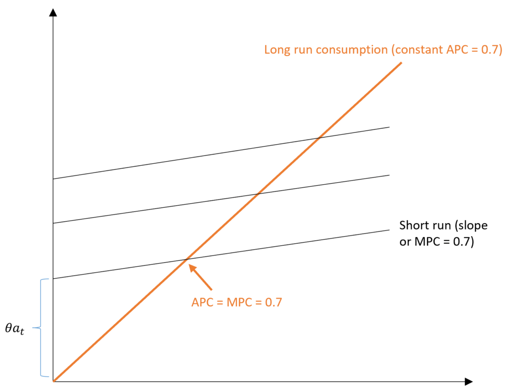
In the long run, however, assets will not be constant. With an increase in assets, the short-run consumption functions will keep shifting upwards as the economy grows. Therefore, long-run consumption will be along the trend where APC is constant and APC=MPC along this long-run consumption.

The APC will be constant if the share of labour income in total income (YtL / Yt) and the ratio of total assets to total income (at / Yt) remain constant in the long run as the economy grows along the trend. Ando and Modigliani observed that both these ratios remained fairly constant in the long run in the annual U.S. data. The labour share in income was around 75 per cent and the ratio of assets to income was around 3. Therefore, the estimated APC is:

criticism of Life-cycle Hypothesis
- The life cycle hypothesis assumes that everyone is a rational consumer aiming to maximize utility based on expected income. However, this may not be necessarily true because not everyone’s consumption decisions are based on future income. Some individuals may not even consider future outcomes while spending in the current period. Or they may be impulsive and lacking in self-control. And, they do not focus on having a smooth consumption over a long period.
- The life-cycle hypothesis assumes that every increase in current income leads to an increase in average future expected income. This may not be true in every case because every income change will not necessarily affect expected future income. For instance, a temporary tax that changes current income, but, consumers are aware that it is temporary and they will not change their expected future income.
Nevertheless, life-cycle theory explains consumer behaviour across cross sections, short run as well as long run. Additionally, it takes into account the role of wealth or assets in determining consumption and can be empirically tested.
Econometrics Tutorials with Certificates
This website contains affiliate links. When you make a purchase through these links, we may earn a commission at no additional cost to you.


T is described as remaining years to life, then why is (T-1) remaining years to employment?
“T-1” is not defined as the remaining years to employment. In the formula, it is the remaining life expectancy of the population.
Sorry, I mistook this website for another one!
That’s alright 🙂