In the long run, firms have a lot more flexibility in the choice of inputs. In addition to labour, firms can choose to expand their capital by setting up new plants and machinery. Or, they can expand the existing plants. Both labour and capital are variable in the long run. As a result, producer equilibrium is determined by considering the costs of both labour and capital.
The goal of a firm is to produce the given output with minimum costs of production. Hence, they will choose a combination of inputs in such a manner that it minimizes their costs. Since both labour and capital are variable, firms will employ that combination of labour and capital which costs them the least, given the prices of labour and capital.
Econometrics Tutorials with Certificates

cost of inputs
We assume perfect competition in the input markets. As a result, the price of labour will be the wage rate. However, the price of capital is a different matter.
We need to compare the cost of capital with the ongoing cost of labour. Therefore, we need to express it in terms of a flow instead of a one-time expenditure of purchasing capital. This is necessary because the cost of labour is a monthly or recurring wage rate. We must express capital in a similar manner for a meaningful comparison. Hence, we express the cost of capital as the “rent” of capital.
Why use Rent as the Price/cost of capital?
This makes sense because capital is often rented instead of purchasing. For capital that is purchased, we consider the “user cost of capital”. This is equal to the “rent” in a competitive market. User cost of capital can be estimated as the sum of depreciation and opportunity cost.
Depreciation is the decrease in the value of capital due to its usage. For instance, consider a firm that buys a piece of equipment for $1000. Its value will not be the same in one year. If the life of that equipment is 10 years, then depreciation would be $100 per year. That is, the value of that equipment will fall by $100 every year and its value will be zero in 10 years.
Opportunity cost can be estimated by considering the interest rate that the firm could have earned instead of purchasing that equipment for $1000. If the interest rate is 5 per cent, the opportunity cost will be 5 per cent of $1000 or $50 in one year. Then, the user cost of capital will be:
User Cost of Capital = Depreciation + Opportunity Cost
User Cost of Capital = 100 + 50 = $150
Rent and user cost of capital are the same under perfect competition because firms earn a competitive rate of return even if they rent out the capital. Therefore, using the capital and the rate at which they will rent the capital will be equal under perfect competition. Rent can, hence, be used as the price of capital to compare with the price of labour.
Isocost line
Isocost line is a locus of all combinations of inputs (labour and capital) that can be purchased at the given total cost. It is similar to the concept of budget line in indifference curve analysis. The budget line shows all the combinations of two goods that can be bought with a given budget by consumers. Whereas, isocost line shows all combinations of two factors that can be bought by the firm given their budget (total cost).
The total cost incurred by the firm to produce any output is the sum of money spent on labour and capital. Hence, the isocost line can be expressed with the following equation:
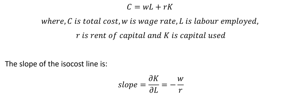
The slope of the isocost line is negative because it is downwards sloping. There is a trade-off between the use of both factors. If a firm wants to use more capital, then the labour employed must be reduced to maintain the same level of the total cost.
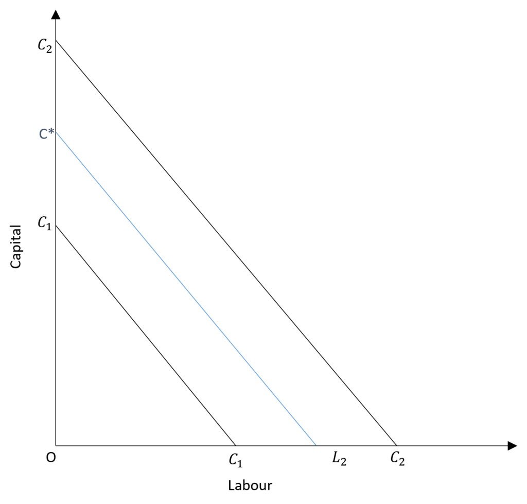
In the diagram, the lines C1, C2 and C* are isocost lines. Each isocost line shows a different level of the total cost. C1 has the lowest total cost and C2 has the highest level of the total cost. All of these isocost lines show different combinations of labour and capital that a firm can employ at different total costs.
producer equilibrium
Suppose a firm wants to produce Q level of output shown by the isoquant Q. Then, the firm will choose a combination of labour and capital which minimizes the cost. That is, the lowest isocost line touching the isoquant Q. Hence, equilibrium will be achieved at the point of tangency of the isocost line and the isoquant. This is shown by E*. At this point, the firm will employ L* and K* levels of labour and capital respectively.
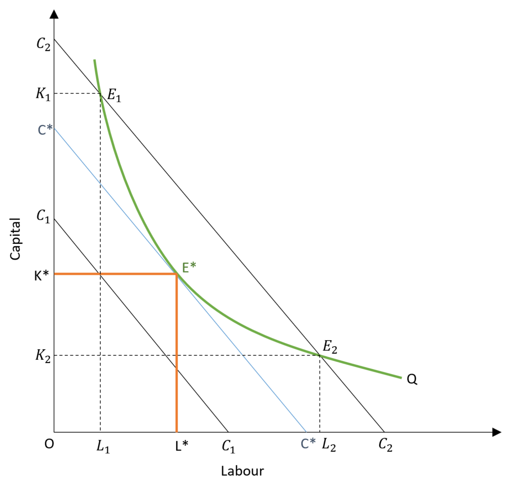
This is the cost-minimizing choice because the other isocost lines either cost more or do not allow the given output to be produced. The isocost line C1 lies below the isoquant implying that the desired output cannot be produced at that cost. On the other hand, the isocost line C2 intersects isoquant Q at two points E1 and E2. However, these points lead to inefficient allocation of inputs because the output Q is produced at a higher cost. Therefore, combinations of L1K1 and L2K2 are not cost-minimizing.
Hence, equilibrium is achieved at E* with L* and K* combination of labour and capital. At this point, the slope of the isocost line and isoquant is equal and tangent to each other.
Slope of Isoquant and Isocost line
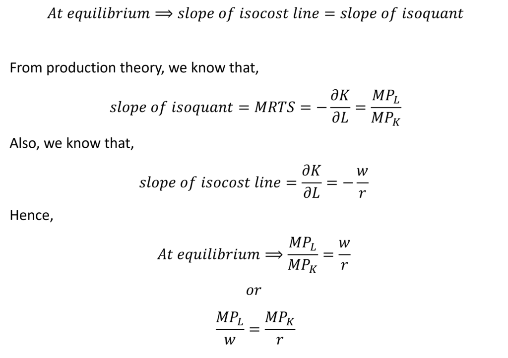
Here, “MPL/w” is the additional output obtained from an additional unit of money spent on labour. And, “MPK/r” is additional output gained from an extra unit of money spent on capital.
At equilibrium, the equalization of these two is achieved because the additional output from the extra dollar spent on each input is the same. Suppose, additional money spent on labour is giving higher additional output. In such a case, a firm will choose to hire more labour because it leads to higher addition in output as compared to capital. As labour increases, its marginal product will fall due to diminishing returns. The additional output per dollar spent on labour will go on falling.
As a result, additional output from extra money spent on labour will go on decreasing till it becomes equal to that of capital. At this point, the firm will stop hiring more labour because the two ratios are equalized. That is, additional output from an extra dollar spent on labour and capital is the same.
change in price of inputs
If the price of an input increases, then a firm will be able to employ less of that input at the given total cost. The effect will be the opposite if the price of input falls and a firm can use more of that input at the same total cost.
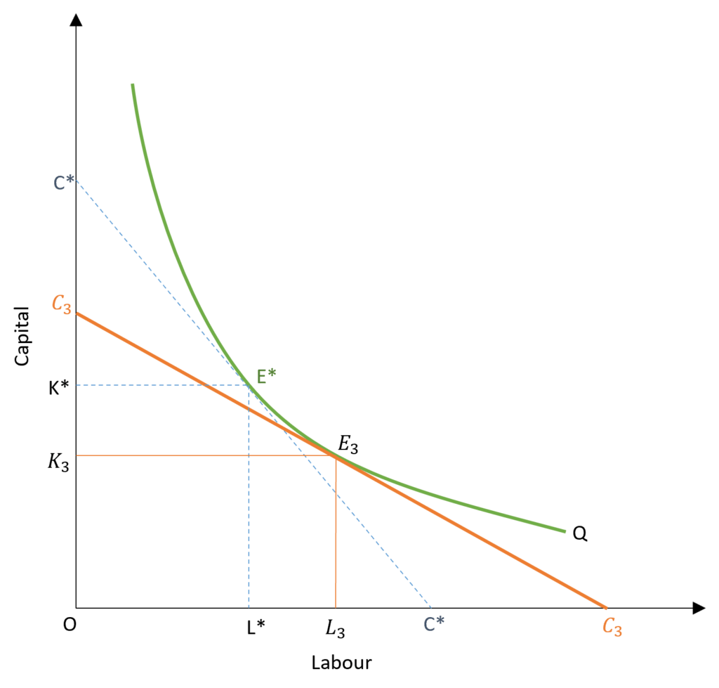
When the price of labour falls and the price of capital rises, the isocost line becomes flatter. Due to a fall in the price of labour, the maximum labour that a firm can hire increases from C* to C3. Similarly, with a rise in the rent of capital, the maximum capital that the firm can rent falls from K* to K3. As a result, the isocost line is a lot flatter or its slope has decreased. If the price of labour increases and the rent of capital falls, the effect is reversed. The slope of the isocost line will increase and it will become steeper.
With a change in the slope of the isocost line, the point of equilibrium will also change. As seen in the diagram, the isocost line is tangent to isoquant at a new point E3. Hence, the cost-minimizing combination of labour and capital changes with a change in their prices and the subsequent shift or change in slope of the isocost line.
Suppose, only the price of labour falls and the rent of capital stays the same. The isocost line will rotate to the right because the firm will be able to hire more labour at the same total cost. This also implies that the producer can operate at a higher output level with the same total cost. Or, they can produce the same output at a lower total cost because labour is cheaper.
Variable output and expansion path
In the above discussion, we focussed on input choice at a given output level. However, firms often change their output levels. They have to adjust the quantity of labour and capital employed to produce that output. As a firm expands its production, they have to employ more labour and capital with technology remaining constant. The equilibrium condition remains the same with a cost-minimizing choice of inputs achieved at the tangency of the isoquant and isocost line.
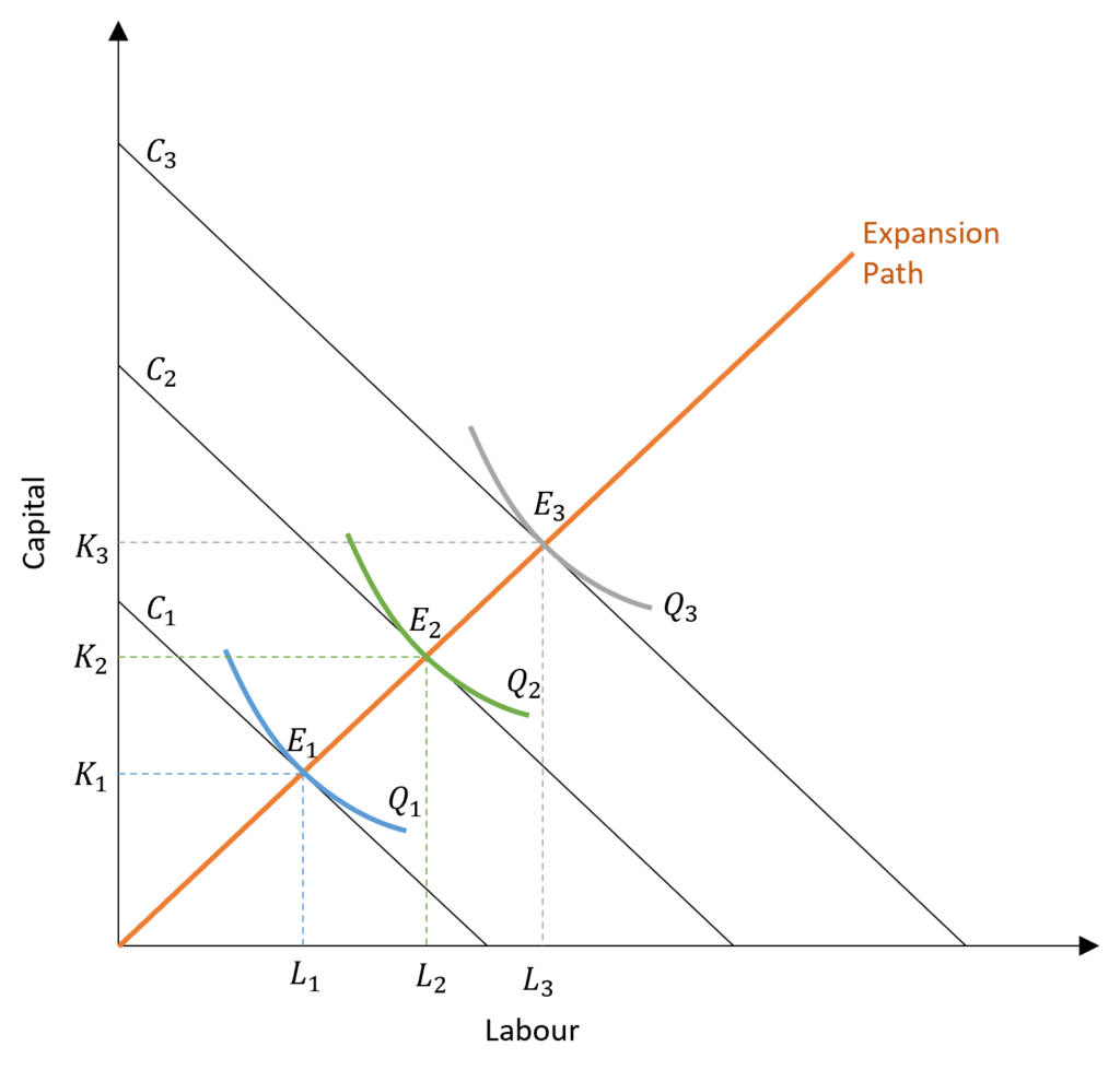
As the firm expands its output from Q1 to Q2 to Q3, the cost of production also rises because more labour and capital need to be used to produce a higher level of output. The cost of production is shown by isocost lines, which keep increasing from C1 to C2 to C3 as output increases. With an increase in output and costs of production, the cost-minimizing or equilibrium level of inputs also increases. Initially, equilibrium is achieved at E1 when output is Q1 and cost of production is C1. At this point, the firm will employ L1 quantity of labour and K1 quantity of capital to minimize costs.
As the firm expands its output level to Q2 and Q3, its cost of production will increase and the equilibrium level will shift to E2 and E3 respectively. Along with this, the cost-minimizing or equilibrium choice of inputs will also shift.
Hence, the expansion path shows the combinations of labour and capital that a firm will employ to minimize costs at every level of output. It joins all the points of tangency between isoquants and isocost lines.
long run total cost from expansion path
The long-run total cost curve can be easily derived from the expansion path. We know the level of output and total cost at all points of tangency or the expansion path.
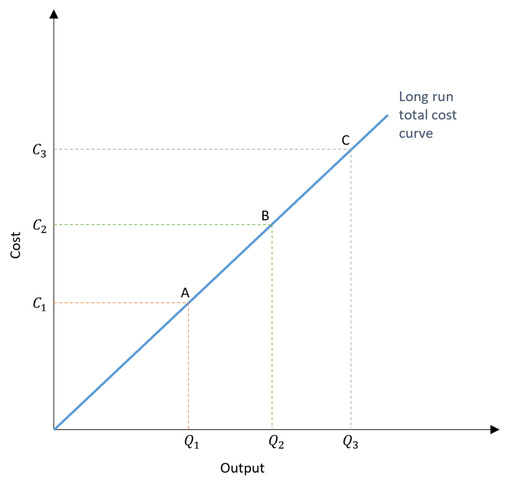
We get the long-run total cost curve by plotting the output and total costs. This shows the change in total cost with the change in output. From the expansion path, we know the costs associated with each output level. When the output is Q1, the cost is C1. Similarly, when output rises to Q2 and then to Q3, the costs rise to C2 and C3 respectively. This gives us the long-run total cost curve.
Important: this straight-line expansion path and straight-line long-run total cost curve assume constant technology. In reality, research and inventions can lead to changing technology over time. We examined the shifts in isoquants with technological change in production theory. Hence, the shape of the expansion path and long-run total cost curve may be determined by the type of technical change or the changing prices of inputs. Technological progress can be neutral, labour deepening or capital deepening. The prices of labour or capital may change over time as well. The equilibrium condition and derivation of the total cost, however, will remain the same.
Econometrics Tutorials with Certificates

This website contains affiliate links. When you make a purchase through these links, we may earn a commission at no additional cost to you.
An exclusive effort from you thanks
Welcome!!!