Similar to the Lewis Model, the structural change theory by Fei and Ranis attempts to explain the transition of underdeveloped agricultural economies with surplus labour into industrialised economies. Furthermore, the Fei and Ranis model borrows heavily from the ideas of Lewis. It extends them further to understand the changes undergone by agricultural and industrial sectors due to structural changes.
Development occurs as surplus labour is reallocated from the agricultural sector to the industrial sector. This process is similar to that of Lewis’ theory. However, Fei and Ranis took this analysis further by examining changes in the agricultural sector. They proposed that structural change will lead to the commercialisation of agriculture with development.
Econometrics Tutorials with Certificates

process of transition
Industrial Sector
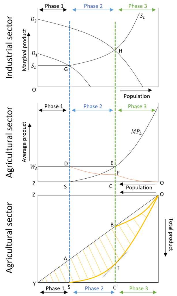
The diagram below depicts the process of transition in both the industrial and agricultural sectors. The top figure shows the marginal product and demand curves of the industrial sector. As in the Lewis Model, the marginal product of labour in the industrial sector is also the demand curve for labour, shown by D1 and D2. The supply of labour is shown by the curve SL, which is horizontal up to point G because of surplus labour in the agriculture sector. The wages and employment are determined by the intersection of demand and supply of labour.
The supply curve SL starts sloping upwards after point G because surplus labour from the agriculture sector is absorbed by the industrial sector. Therefore, more labour is supplied only at higher wages. As a result, wages will rise and the supply curve will be upward sloping after the surplus labour is depleted from the agricultural sector. With an increase in capital, the marginal product and the demand curve will shift upward from D1 to D2 as development occurs. This will also expand the industrial sector and its employment.
Agriculture Sector
The bottom two figures of the diagram show the process of transition in the agricultural sector. Initially, the economy is operating at point Y in the last figure. The amount of surplus labour is equal to SY at this point. With development, this surplus labour shifts from agriculture to the industrial sector. Because of the existence of surplus labour, the total product does not fall in the agriculture sector. The OS curve shows the total product, which reaches the maximum at point S and does not increase beyond that point because of surplus labour.
The wages in the agricultural sector are not determined by its marginal product. Wages are equal to the slope of OY (which is ZY / OY). These real wages are fixed due to institutional factors because the wages will fall to 0 if determined by marginal product because the marginal product is 0 due to redundant labour. Hence, institutional wages are fixed at WA shown in the second figure.
The rise in wages
The wages in the agricultural sector will start rising as labour is reduced beyond point C. At this point C, the institutional wages WA will be equal to the competitive wage level as shown by point T. Point T is tangent to the total product curve. Beyond this point, wages will be determined by market forces as they rise above institutional wages.
The quantity of labour YC is referred to as disguised unemployment in the agricultural sector. This is because the marginal product of labour is below the institutional wages (WM > MPL) as more labour is employed. This is evident in the second part of the diagram. The marginal product curve falls below the wage level when labour is greater than point C and the MPL curve reaches zero at point S (total product reaches the maximum in the third diagram).
Shortage and commercialization point
Shortage Point
Point S in this transition is called the shortage point because the average agricultural surplus (AAS) starts falling as labour reduces in the agricultural sector. The total agricultural surplus (TAS) is still rising at this point. TAS is shown by the shaded region in the third diagram and the AAS is shown by the curve WADFO in the second diagram.
As seen in the diagram, the total agricultural surplus will increase in Phase 1. However, TAS starts falling as labour falls lower than S. Here, AAS also starts to fall as shown by the DF portion of the curve. Because the average agricultural surplus available starts decreasing, point S is called the shortage point as the agricultural sector starts developing a shortage of surplus.
Commercialization Point
Point C in the diagrams represents the commercialization of agriculture. This is because the wages in agriculture will start rising as the shortages in AAS increase (shown by the fall in AAS in portion FO of the curve) rapidly with a decrease in labour below point C. The landowners will be willing to pay more for agricultural labour. On the other hand, industrial sector wages will also have to increase more to attract agricultural labour beyond this point.
Hence, this point represents a landmark in the development process because the agriculture sector is commercialised. There is no disguised unemployment with excess labour transferred to the industrial sector.
| Phase | Agricultural sector | Industrial sector | Total agricultural surplus (TAS) | Average agricultural surplus (AAS) |
| Phase 1 | Institutional wage WA | Constant wages as surplus or redundant labour are being absorbed | Increasing TAS | AAS equal to the institutional wage |
| Phase 2 | S = shortage point Institutional wage WA | Wages start rising because surplus labour has been removed from agriculture YC = disguised unemployment in the agriculture sector | TAS still rising | AAS starts declining leading to shortages in output surplus |
| Phase 3 | C = commercialization point Wages start rising | Wages keep increasing | TAS starts falling | AAS declines rapidly |
Criticism
- Institutional Factors: surplus labour is not the only reason that explains the underdevelopment of the agriculture sector in certain economies. In many cases, it has been observed that underdeveloped economies do not have surplus labour in the agriculture sector. Some institutional factors, such as feudal structure, prevailing within these economies are the major reason behind their underdeveloped agriculture sector.
- Zero marginal product: the assumption of zero marginal product of labour in phase 1 has been heavily criticized. When labour shifts to the industrial sector initially, the Total product does not fall in the agriculture sector. For MPL to be zero, the agricultural labour has to be very large. Various studies have shown that this assumption does not hold in reality.
- Capital-intensive technology: as seen in the Lewis Model, the growth in the industrial sector may not necessarily lead to a shift of labour from agriculture to the industrial sector. With technological progress, the industrial sector may witness the development of capital-intensive technology. In this case, the industrial sector will grow but without any additional employment of labour.
Econometrics Tutorials with Certificates

This website contains affiliate links. When you make a purchase through these links, we may earn a commission at no additional cost to you.