Seasonality, sometimes referred to as seasonal variation, is common in economic time series. The time series variables may change in a cyclical pattern with time. This cyclical pattern is termed seasonality and can be estimated using Seasonal-ARIMA (SARIMA) models.
For instance, consider the behaviour of the tourism industry of a hill station. It will see a rise in tourism during the summer months and a subsequent fall during winters. This makes a cyclical pattern with a peak during summers and a trough during winters. In other words, tourism activity in a hill station will be high during summers and low during winters. This cycle is repeated each year with time, showing a wave-like pattern in the time series.

In practice, economic time series often show this type of behaviour. In some cases, seasonally adjusted time series are available where the seasonality has been removed from the variables. However, this may not be possible or desirable in every situation. In some cases, we need to explicitly analyse and understand seasonal behaviour.
Moreover, the pattern of seasonality may depend on the type of data. In a monthly time series, a seasonal cyclical pattern may repeat every 12 time periods because we have 12 months in a year. Similarly, a quarterly time series may repeat its pattern every 4 time periods because we have 4 quarters in a year. In addition, we may even need to model multiple seasonal patterns in some rare cases.
recognising seasonality: additive v/s multiplicative seasonality
The seasonal behaviour of a time series variable may be either additive in nature or multiplicative. It is essential to distinguish between the two because they need to be handled differently.
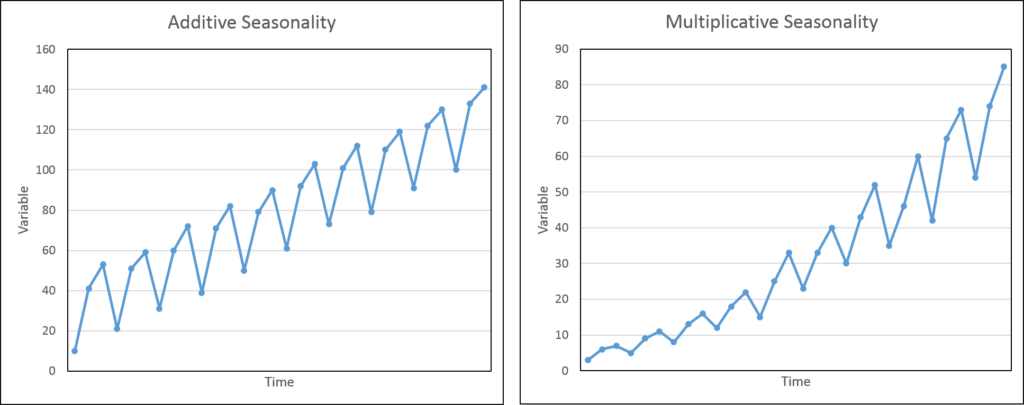
Additive seasonality is a situation where the magnitude of the cyclical pattern remains the same with time or trend. With the passage of time or the falling/rising of trend in the variable, the magnitude of the cyclical pattern does not change. This means that the height of the peaks and the depth of the troughs remain more or less the same. This type of seasonal behaviour can be modelled using basic ARIMA models. We can either introduce seasonal dummies or AR and MA terms based on the seasonal cycle in the ARIMA model as needed.
Multiplicative seasonality refers to the seasonal behaviour that changes its magnitude with time or trend. With an increase in the trend, the magnitude of seasonal cycles also increases. Conversely, the magnitude of seasonal variation falls with a falling trend. This implies that as the trend increases, the peaks in the cyclical pattern become higher and the troughs become deeper. It is known as multiplicative because the relationship between trend and seasonality is multiplicative. That is, the higher the trend, the higher will be the seasonal cyclical variation.
We can usually recognise whether seasonality is additive or multiplicative by plotting the variable against time:
Pattern of seasonality and seasonal lag: example
ARIMA and SARIMA models are often used to model data with seasonal variations. We can use ARIMA models for Additive Seasonality and SARIMA (Seasonal-ARIMA) models for Multiplicative Seasonality.
Here, we will consider a quarterly time series of consumption. The data is not seasonally adjusted, which means that we may find seasonal variations in the time series. First, we need to figure out if there is seasonality in the data. If seasonality is present, we need to decide on the seasonal lag (length of 1 seasonal cycle). Since that data is quarterly, we expect that the seasonal lag maybe 4, i.e. seasonal cycle will repeat after every 4 time periods. Let us look at some time series plots of the data:
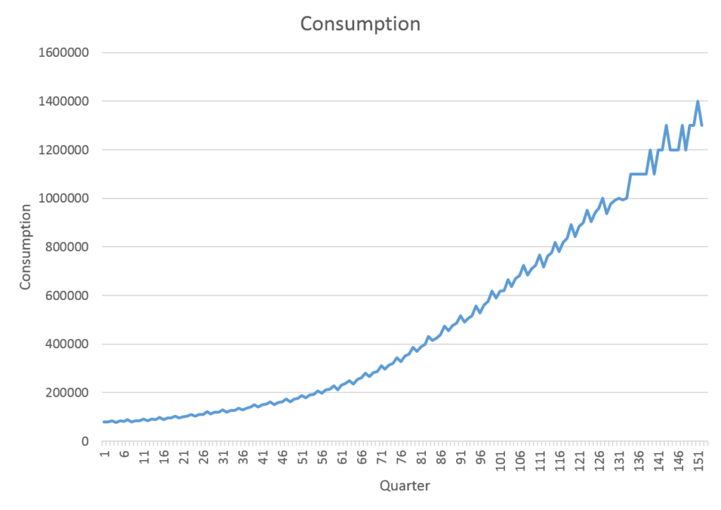
Looking at the graph, there is a strong indication of multiplicative seasonality. As we can see above, the magnitude of seasonal cycles goes on increasing with the trend. This suggests a multiplicative relationship between trend and seasonality.
Choosing AR, MA, seasonal differencing, seasonal AR and Seasonal MA terms
Stationarity, Order of Integration and seasonal differencing
As in the basic ARIMA models, the first step is to determine the order of integration of the time series. The time series of consumption used in the graph above is non-stationary at levels. Using the ADF test, we can determine the Order of Integration of the series. In this example, the consumption is non-stationary at level but stationary at first differences. Therefore, the Order of Integration is one (d = 1). Now, we know that the series must be differenced once in the ARIMA model.
As for seasonal differencing, we can account for additive seasonal effects with the help of seasonal differences or by including AR or MA terms at the seasonal lags. For instance, we can include AR(4) or MA(4) terms as needed to account for seasonal effects in quarterly data. We can also use seasonal difference (Ct – Ct-4) to eliminate additive seasonality.
In this example of consumption, these measures will not be enough because the seasonality is multiplicative. Instead of AR and MA seasonal terms in ARIMA, we will have to estimate a SARIMA model. Since the series is stationary without taking seasonal differences, we will initially approach without seasonal differencing. Later, we will compare the two SARIMA model, with and without seasonal differencing, for their forecasting power.
Choosing AR, MA, Seasonal AR and Seasonal MA lags
The autocorrelation function (ACF) and partial autocorrelation function (PACF) can give us a good starting point for the lags we need to include. We expect that we will need to use the SARIMA model because of multiplicative seasonality. Let us look at the ACF and PACF of the series (at first difference because d = 1):
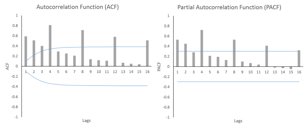
As expected, we can clearly observe a seasonal cycle of 4 time periods. Both the ACF and PACF show a significant value after every 4 lags. The ACF is falling gradually after every 4 lags and we can observe the same for PACF. This suggests that we may need AR and MA seasonal lags.
For the ARIMA component, we may include AR(1) and MA(1) as the first lags of ACF and PACF are significant and gradually falling.
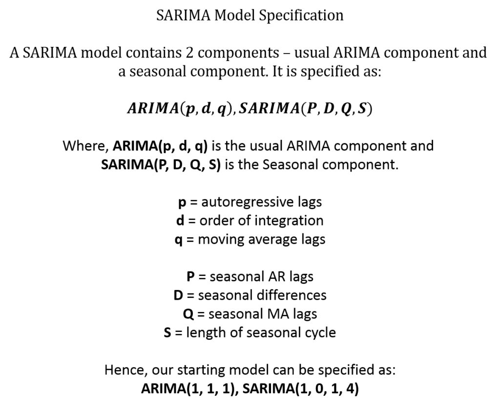
From this behaviour, a SARIMA model with (1, 1, 1) ARIMA component and (1, 0, 1, 4) Seasonal component seems like a good starting point. The specification of SARIMA has the following components:
SARIMA estimation, forecasting and choosing the best model
SARIMA models can be estimated easily with the help of statistical software packages. They are non-linear in nature and are estimated using the Maximum Likelihood technique. The SARIMA model we specified above is a good starting point. We can compare this model with other SARIMA specifications and decide the final model specification based on which model gives the best results.
For this purpose, we can use various information criteria to choose the best model. As we did in the basic ARIMA model estimation, we can employ AIC and SIC to choose the model with the minimum value of these information criteria. Or, we can choose the model that gives us the best forecasting performance.
Generally, SARIMA models are used for forecasting purposes. Therefore, we will choose the model with the best forecasting performance here.
Results of Seasonal-ARIMA (SARIMA)
| SARIMA Specification | Overall Forecasting Error (%) | Dynamic Forecasting Error (%) |
| ARIMA (1, 1, 1) | 6.97 | 11.48 |
| ARIMA (1, 1, 1), SARIMA (1, 0, 1, 4) | 1.74 | 2.32 |
| ARIMA (1, 1, 1), SARIMA (1, 1, 1, 4) | 1.06 | 1.18 |
| ARIMA (1, 1, 1), SARIMA (2, 1, 1, 4) | 1.06 | 1.16 |
| ARIMA (1 3, 1, 1), SARIMA (1, 1, 1, 4) | 3.72 | 8.83 |
| ARIMA (1 3, 1, 1), SARIMA (2, 1, 1, 4) | 3.84 | 9.26 |
We have included the results of the basic ARIMA (1,1,1) for reference. As expected, it does not perform well because it does not consider seasonal variations at all. Among our SARIMA models, the model with two seasonal AR lags, one seasonal difference and one seasonal MA lag is performing the best. This is clear because it has the minimum forecast error. Even for dynamic forecasts, this model has a small error of 1.16 per cent. This model is specified as ARIMA(1,1,1), SARIMA(2,1,1,4). The ARIMA (1,1,1), SARIMA (1,1,1,4) is also performing as well as the model with 2 seasonal AR lags.
The last 2 models have a more complicated specification as they include 1st and 3rd lag in the ARIMA component. These models are not performing well, but they show the flexibility of ARIMA and SARIMA model specifications. If needed, we can even include multiple seasonal behaviours in the model.