The usual Goodness-of-fit statistics such as R-square and Adjusted R-square are not applicable in the case of Qualitative Response models. This is because the Ordinary Least Squares method of estimation is not appropriate for these models. As a result, a different set of statistics must be used to assess the reliability of the Logit and Probit models (Qualitative Response Models). Here, we will discuss the application and interpretation of Goodness-of-fit for Logit and Probit Models. We will focus on the implementation of Classification Tables, Count R-square, McFadden R-square, Pseudo R-square and Likelihood-Ratio test.

Specification of the Logit or Probit Model
The dependent variables are not always continuous or quantitative. We often deal with dependent variables that are qualitative in nature, where we have a categorical dependent variable instead of a continuous variable. The application of Ordinary Least Squares to such models is referred to as Linear Probability Model (LPM). The LPM, however, has serious drawbacks and is not generally used for models with categorical dependent variables. Similarly, the Goodness of fit statistics used after OLS are not applicable. As a result, we employ Logit or Probit models for estimation and a different set of goodness of fit measures.
To illustrate the use of Goodness of fit statistics for Qualitative Response models, we will consider the following model:
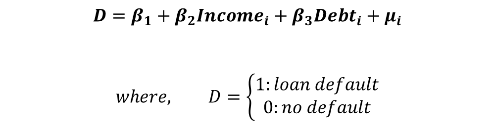
The dependent variable takes the value of 1 in case of loan default and 0 if the person does not default. We will consider two independent variables of income and credit debt. Using Logit and Probit models, we can analyse the effect of income and credit debt on the probability of loan default.
Results of Logit Model
The Logit and Probit models are estimated using the Maximum-Likelihood technique. Here, we will present the results of the Logit model only. The associated likelihood functions and derivation of marginal effects are available there as well.
| Log-Likelihood = -33.893396 | ||||
| Dependent variable – Defaulter | ||||
| Independent Variables | Coefficient | Standard Error | Z | p-value |
| Income | -0.0465985 | 0.210198 | -2.22 | 0.027 |
| Debt | 0.7407529 | 0.2833296 | 2.61 | 0.009 |
| Constant | -0.4684091 | 0.5642932 | -0.83 | 0.406 |
The important thing to note here is that the coefficients do not show the effect of these variables on the probability of loan default. Instead, they show the relationship between variables and log-odds. The log-odds interpretation does not make much economic sense in this form. We can only ascertain whether the coefficients are significant or not. Hence, we calculate the “Marginal Effects” after estimation:
Marginal Effects
| Y = Pr(defaulter) (predict) = 0.20788562 | |||||
| Independent Variable | Marginal Effects | Standard Error | Z | p-value | Mean Value |
| Income | -0.0076733 | 0.00319 | -2.41 | 0.016 | 42.2 |
| Debt | 0.1219792 | 0.0438 | 2.78 | 0.005 | 1.5 |
This table shows the “Marginal Effects at Mean”. At mean values of independent variables (mean income = 42.2 and mean debt = 1.5), the probability of default is 0.20788562.
We can observe a negative relationship between income and the probability of default because there is a negative sign alongside the marginal effects. If income increases from its mean by a small amount (other variables constant at their mean), the probability of default falls by 0.76733 per cent. This negative relationship makes sense because an individual with a higher income is less likely to default on a loan.
Similarly, the relationship between debt and the probability of default is positive. That is, an increase in debt increases the probability of default, which is expected. An increase in debt by a small amount (other variables constant at mean) from its mean leads to an increase in the probability of default by 12.19792 per cent.
Goodness-of-fit statistics and their interpretation
Classification Table
The Logit and Probit models give us the probability of default. We can use that probability to classify each individual as a defaulter or not a defaulter. For instance, we can decide the probability cut-off to be 0.5. Then, individuals having a probability of default higher than 0.5 are classified as defaulters. Individuals with a probability equal to or lower than 0.5 are considered as ones who will not default.
Because we already know whether an individual is a defaulter or not (from the data), we can assess how well our model is classifying or identifying the defaulters using the estimated coefficients and probabilities.
| Cut-off = 0.5 | True | |||
| Logit Model | + | – | Total | |
| + | 1 | 2 | 3 | |
| Classified | – | 16 | 51 | 67 |
| Total | 17 | 53 | 70 |
Out of the total of 70 individuals or observations, our model classified 52 of them accurately. This gives us a 74.29 per cent accuracy. We can see the correct predictions in the diagonal elements of the table which shows 1 True Positive and 51 True Negatives, making a total of 52 correct classifications.
True Positives, True Negatives, False Positives and False Negatives
The true positives refer to the observations that were classified as defaulters and were defaulters in real data. True negative implies observations that were classified as not being a defaulter and were not defaulters in real data.
The wrong classifications are shown by False Positives and False Negatives. False Positives mean that observations were wrongly classified as defaulters, but, were not defaulters in real data. Our model shows 2 False Positives according to the table.
False Negatives refer to observations that were wrongly classified as not being defaulters when they were defaulters in the real data. The table above shows that our models have 16 False Negatives.
Although our model has an accuracy of 74.29 per cent, it is not performing too well in identifying defaulters. This is evident from a large number of False Negatives, i.e. our model is struggling to identify individuals who are defaulters and is classifying them as not being defaulters.
Using the cut-off in Classification tables
Suppose, our priority is to recognise Loan Defaulters (high True Positive and low False Negative), even if we end up wrongly classifying some of them as defaulters (high False Positives). Hence, we are willing to tolerate high false positives to have low False Negatives. To achieve this, we can lower the cut-off below 0.5 so that we do not miss any potential defaulters.
For instance, we can have the cut-off at 0.4, which means that individuals with a probability of default above 0.4 are classified as defaulters. Let us look at the results:
| Cut-off = 0.4 | True | |||
| Logit Model | + | – | Total | |
| + | 5 | 3 | 8 | |
| Classified | – | 12 | 50 | 62 |
| Total | 17 | 53 | 70 |
From this table, we can see that the True positives have increased to 5 and False Negatives have decreased to 12. Hence, with a cut-off at 0.4, our Lobit model is doing better at identifying defaulters. Even the overall accuracy has increased to 78.57 per cent from 74.29 per cent at 0.5 cut-off.
Hence, the choice of cut-off has a huge impact on the classification accuracy and must be chosen carefully. The choice of cut-off will depend on the priority of the research. For example, we wanted to identify defaulters and decided to lower the cut-off to 0.4 so that we do not miss any potential defaulters due to the high cut-off (0.5).
In the example we have considered, the accuracy of 78.57 per cent might not be satisfactory. We can improve the model further by including more independent variables that affect the probability of default. For instance, the wealth of an individual or the number of years in employment can play a massive role in determining whether an individual will default on a loan or not.
Count R-square

This is similar to the accuracy that we calculated in the classification table. For the 74.29 per cent accuracy that we calculated earlier at 0.5 cut-off, the Count R-square will be 0.7429.
McFadden R-square

This measure is used to compare and choose between two models. A model with a higher value of McFadden R-square is preferred. Generally, a value between 0.2 and 0.4 of McFadden R-square is considered acceptable.
Pseudo R-square
Cragg, Uhler, and Maddala suggested another measure known as Pseudo R-square which can be estimated as follows:
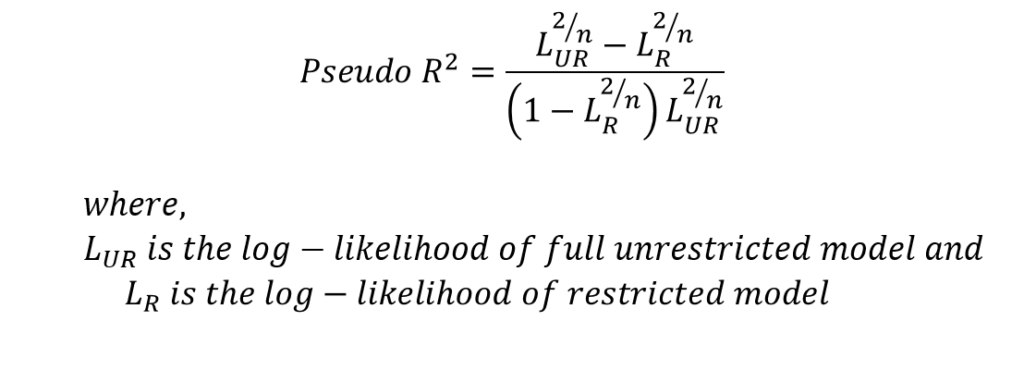
Similar, to McFadden R-square, this measure is used to compare two models. The model with a higher value of Pseudo R-square is preferred.
Likelihood-Ratio test

The LR statistic follows the chi-square distribution and the model is a good fit if it is observed to be statistically significant. This test compares a restricted model (only constant) with a model including all independent variables (unrestricted model). If the LR statistic is significant, we conclude that the inclusion of independent variables results in a better fit.
For the application of Goodness of fit statistics after the OLS model in R, you can check out Goodness of fit in Rstudio.