Blog

The expansion of output can be accompanied by increasing, constant or decreasing returns to scale. These can also correspond to Economies of scale. As discussed in production theory, returns to scale determine the shifts in isoquants.

Constant Returns to Scale

Constant returns to scale imply that when output is doubled, the costs will also be doubled. That is, the rate of increase in output is accompanied by an equal rate of increase in the cost of production. Suppose, an increase in output from 20 to 40 units is accompanied by an increase in cost from 10 to 20 dollars. Then the firm is experiencing constant returns to scale.

Increasing Returns to Scale

Increasing returns to scale occur when the rate of increase in output is greater than the rate of increase in the cost of production. For example, if the increase in output from 20 to 40 units is accompanied by an increase in cost from 10 to only 15 dollars. Or, doubling costs from 10 to 20 dollars leads to more than double the output from 20 to 50 units. In that case, the firm is witnessing increasing returns.

Decreasing Returns to Scale

Decreasing returns to scale is the opposite of increasing returns. The rate of increase in output is less than the rate of increase in the cost of production. For instance, an increase in output from 20 to 30 units when cost increases from 10 to 20 dollars is an example of decreasing returns. Or, to double the output from 20 to 40 units, the requirement of more than double the cost from 10 to 30 dollars is also an example of decreasing returns.

These are discussed in more detail in Isoquants and returns to scale.

This website contains affiliate links. When you make a purchase through these links, we may earn a commission at no additional cost to you.

economies and diseconomies of scale

Economies of scale

Diseconomies of scale

With large output, firms need to buy inputs and raw materials in bulk. This allows them to negotiate better prices and avail the extra benefits of buying in huge quantities. The expansion allows increased specialization of the labour force. Workers can be assigned to activities in which they are most productive. The increased scale provides better flexibility and a chance to make the production process more efficient.

Beyond a certain point of expansion, inefficiencies can start to show because managing a huge firm becomes difficult with the increase in the number of tasks to handle and the communication gap due to the massive size of the workforce. The benefits of purchasing raw materials or inputs in large quantities may disappear as inputs are not unlimited. Eventually, a shortage of inputs will increase their costs.

Difference between Returns to Scale and Economies/Diseconomies of Scale

Returns to scale apply when the input proportions remain the same. That is when the inputs are used in the same proportions even when more or less of them are employed. If the input proportions change, we do not refer to it in terms of the returns to scale. But, we use the term economies or diseconomies of scale. To make this clear, let us consider an example of a clothing firm.

Suppose, a clothing firm uses labour and some equipment to knit sweaters. To expand their production, the firm will need to employ more labour and knitting equipment for that labour. If they expand production, labour and knitting equipment will have to expand together. The firm will experience constant returns to scale because labour productivity is not changing and extra labour and equipment will increase output in the same proportion. This is an example of constant returns to scale when a doubling of costs of production (due to double labour and knitting equipment) leads to a doubling of output.

However, firms also have an option for expansion using more efficient and specialised machines with different labour requirements to make sweaters. If they use new specialised machines instead of increasing existing knitting equipment and labour, then input proportions will change. Doubling output, in this case, will require less than double the increase in the cost of production due to specialised machines. The firm will experience economies of scale.

Long run average cost and marginal cost

In case of constant returns to scale in the long run, the long-run average cost curve (LAC) would be a straight line parallel to the x-axis. This happens because the rate of increase in output is the same as the rate of increase in cost. Therefore, the average cost (TC/Q) will be constant. Moreover, the long-run marginal cost curve will also be constant and equal to LAC.

However, firms do not operate on constant returns to scale. Instead, firms experience increasing returns to scale when they start expanding. This happens due to the economies of scale. Hence, the LAC will decrease in the beginning when output expands because the increase in output is greater than the increase in costs. As they go on expanding the output, diseconomies of scale start to appear. As a result, LAC will start to slope upwards with decreasing returns to scale.

U-shaped LAC

LAC is U-shaped, which is similar to the short-run average cost curve. But, the reason for this shape is increasing and decreasing returns to scale or economies and diseconomies of scale. In the short run, a U-shaped average cost curve (ATC) occurred due to diminishing returns to a factor.

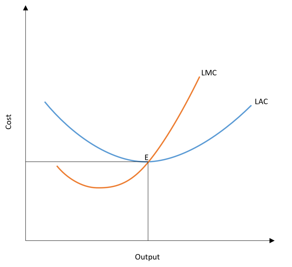
Long run marginal cost curve (LMC) is derived from the long-run total cost curve. It shows the increase in total cost with a one unit increase in output. Similar to the short run, when LAC is downward sloping, LMC is less than LAC. LAC starts sloping upwards when LMC becomes greater than LAC. Therefore, LAC is at its minimum when LAC = LMC.

long run vs short run expansion

In the short run, not all inputs can be varied. Expansion in factors such as capital equipment requires a longer period of time. Therefore, capital is constant in the short run and variable only in the long run. As a result, long-run production provides more flexibility in the expansion of output through various combinations of inputs. On the other hand, short-run production can be inflexible because the expansion of output can only take place by increasing labour.

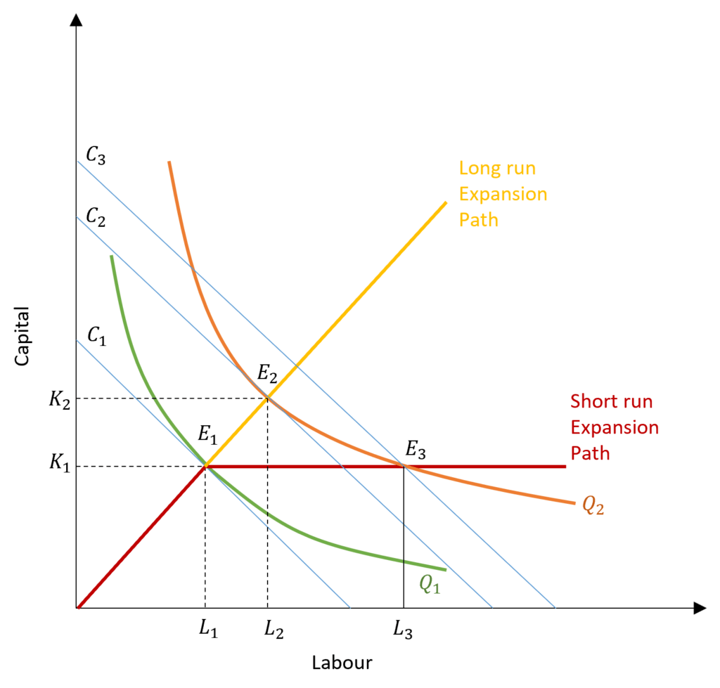
In the diagram, we can observe that output can be increased to Q₂ by increasing cost to isocost line C₂. A firm can achieve this by employing more labour as well as capital in the long run. However, short-run expansion is inflexible because capital is constant. Therefore, to increase output from Q₁ to Q₂ in the short run, a firm must incur higher costs shown by isocost line C₃. This happens because the firm cannot increase its capital above K₁ and have to operate at a higher isocost line, which is not a cost-minimizing combination of capital and labour. The cost-minimizing isocost line is C₂ for the output of Q₂, where the firm will operate in the long run.

The short-run expansion path is, therefore, different from the long-run expansion path. Short run expansion path shows the firms’ inflexibility in the short run. In the beginning, the short-run expansion path is upward sloping and similar to long-run expansion till it reaches the K1 amount of capital employed. After this point, capital cannot be increased in the short run. The short-run expansion path becomes a constant or straight line parallel to the x-axis.

relationship between long run and short run costs

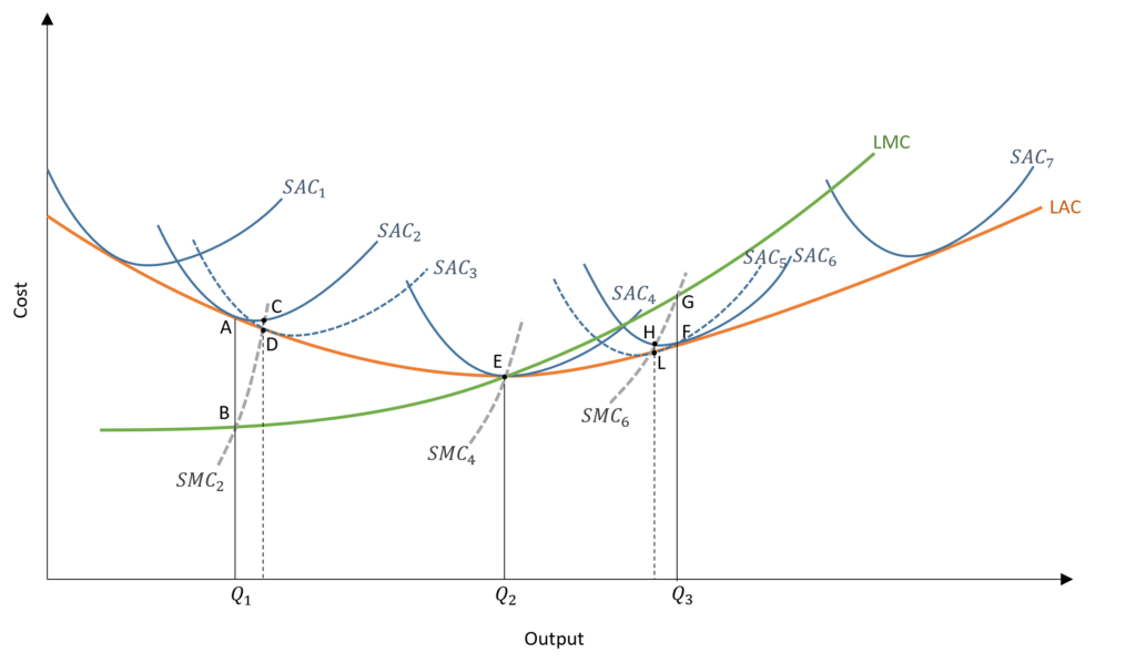
The LAC shows long-run average cost, which decreases when the firm expands its scale initially because of economies of scale. After Q₂ output, the LAC is upward sloping due to diseconomies of scale as the firm expands. The LAC, therefore, represents the average cost when the firm grows in scale. The short-run cost curves (SAC₁ to SAC₇) show short-run average costs at every scale of operation of the firm.

Hence, a firm faces different short-run average cost curves at every point of its expansion. That is, the SACs depict the average costs at every different plant size. As the firm increases its scale of operation by setting up new plants and purchasing new equipment, the firm will face different average cost curves in the short run from SAC₁ to SAC₇. Hence, the LAC is an envelope of the short-run average cost curves (SACs) which lie above the LAC.

Choice of Operation

At Output Q₁

The firm will choose the scale of operation based on the tangency of LAC and SAC. Suppose, the firm wants to produce Q₁ output. Then, the firm will choose the scale of the firm shown by SAC₂ because it is tangent with LAC at that output, shown by point A. It is important to note that this is not the minimum point of SAC₂ and it reaches its minimum at point C where SMC₂ or short-run marginal cost curve cuts it from below.

However, the firm will not operate at this minimum point because it will have to forego economies of scale if the firm chooses to operate at C. This happens because the firm can reduce its average cost by expanding its scale. This is evident from the fact that the LAC lies below point C. Therefore, firm can reduce its cost by expanding and operating at the tangency of SAC₃ and LAC, as shown by point D. The difference between point C and point D is the amount by which the firm can reduce its average cost by expanding to SAC₃ and get some economies of scale.

At Output Q₃

This same strategy is applicable if the firm wants to produce Q₃ quantity of output. Then, the firm will operate on SAC₆ which is tangent to the LAC (point F) corresponding to Q₃ level of output. The minimum point of SAC₆ is at point H, where SMC₆ cuts it from below. But, the firm will not operate at this minimum point because it can reduce its average cost by producing at a smaller scale shown by SAC₅. The difference between point H and point L is the amount by which the firm can reduce its average cost by producing at a lower scale shown by SAC₅.

Long-run and Short-run Marginal Costs

At point E, all the curves pass through the same point. LAC, SAC, SMC and LMC are equal at E. This happens because it is the minimum point of LAC as well as SAC₄. After this scale of operation, the LAC will start to slope upwards and the firm will observe diseconomies of scale by expanding plant size and equipment.

We have seen that LAC is an envelope of short-run average cost curves. But, this is not true for LMC or the long-run marginal cost curve. LMC is not an envelope of SMCs (short run marginal cost curves). Instead, each point on LMC shows the SMC at every cost-efficient plant size. For instance, we established that firm will operate at SAC₂ to produce Q₁ output. The SMC₂ intersects LMC at point B corresponding to the tangency of LAC and SAC₂. This shows the cost-efficient plant size to produce Q₁. The same is true for SMC₆ which intersects LMC at point G. This shows that the LMC consists of all the points of SMCs which correspond to efficient or cost-effective production.