The Logit Model is used to estimate models with a qualitative binary dependent variable. It overcomes the problems associated with the Linear Probability Model (LPM). In the post on LPM, we discussed that the application of OLS is not appropriate when we have a binary or qualitative dependent variable.

Firstly, the probability from the Linear probability model (LPM) might exceed the limits of 0 and 1. A negative or greater than 1 probability does not make sense. Secondly, the residuals from the LPM are heteroscedastic. This violates a key assumption of OLS and the tests of significance become unreliable or invalid.
Finally, LPM assumes a linear relationship between the independent variables and the binary dependent variable. This assumption is unrealistic because the change in probability should be slow or small at extreme values of independent variables. That is, with a small change in independent variables, the change in probability should be different at different levels of those independent variables. This implies a non-linear type of relationship between the independent and dependent variables.
Logit Model and Sigmoid Function
The Sigmoid Function is used in the Logit Model to overcome the problems in the Linear Probability Model. The Sigmoid function ensures that the probability does not exceed the limits of 0 and 1. Moreover, the Sigmoid function is non-linear. As we approach extreme levels or values of independent variables, the change in probability due to a small change in the independent variable keeps getting smaller and smaller.
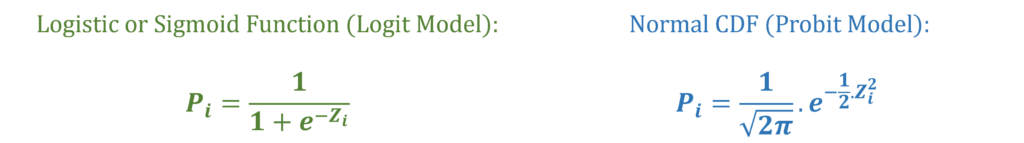
Both the Sigmoid function and the Normal Cumulative Distribution Function fulfil these criteria. The Sigmoid function is used in the Logit Model, whereas, the Normal CDF is used in the Probit Model. Let us take a look at the general structure and shape of these functions:
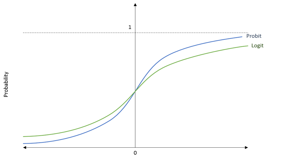
In the diagram, we have the probability (Pi) on the y-axis and the value of Zi on the x-axis. This Zi is a value that enters the Sigmoid function or the Normal CDF as we can see in the formula above. In the Logit and Probit Models, we get this value Zi from the independent variables in the model.
If we look at the shape of the functions, we can see that they never cross the limits of 0 and 1. They keep getting closer to these limits, but they never touch them. This also means that the functions become flatter as we move towards the extreme values on the x-axis. That is, the change in probability is smaller or slower at the extreme values on the x-axis. This is exactly what we need to deal with the problems we discussed in the LPM.
Logit Model Estimation
Let us consider the same simple model that we stated in the Linear Probability Model:

The dependent variable X is binary and is equal to 1 if the individual owns a car. The value of X is 0 if the individual does not own a car. Moreover, X is a function of the independent variable income or Yi. But, we should not estimate this model with OLS. Instead, we will use the Sigmoid function to modify this model and apply the Logit Model. The Sigmoid function is used to project this model equation as follows:
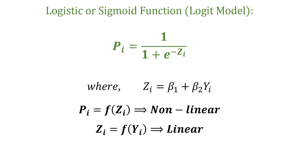
In the function, the coefficients and the independent variable income (Yi) give us the value of Zi. In turn, Zi in the Sigmoid function gives us the probability (Pi). Further, we can observe that Zi is still a linear function of the independent variables. However, the Probability (Pi) is a non-linear function of Zi.
Maximum Likelihood Method
With the help of the Sigmoid function, we have a formula for Pi stated above. This is used to derive the Likelihood and also the Log-likelihood functions under the i.i.d assumption. That is, the model assumes that the observations are identically and independently distributed. For a complete derivation of the Likelihood Function for the Logit Model and details about its assumptions, you can see the Video Tutorials on Logit and Probit Models. The final log-likelihood for the Logit Model can be expressed as:

We estimate the coefficients of the model by maximizing this log-likelihood with respect to the parameters of the model (β1 and β2 in this example). The logic behind the Maximum Likelihood approach is that we have to obtain the values of parameters in such a way that the probability of observing the sample values of X is at the maximum.
Interpretation of the Coefficients
The interpretation of the coefficients from the Logit model does not make much economic sense. This is because it shows changes in log odds with a change in the independent variable. In our example, with a 1 unit increase in income, the log odds of car ownership will increase by β2. This explanation can be derived as shown in the Video Tutorials on the Logit and Probit Models and can be expressed as:

Here, Pi is the probability of success or the probability that the individual owns a car. Similarly, “1 – Pi” is the probability of failure or not owning a car. This Pi divided by “1 – Pi” is known as the odds of the event. Therefore, taking the natural log means that the above formula is for the log odds of owning a car. The log odds are a function of the independent variables in the model, income (Yi) in this example. Hence, a unit change in income leads to a β2 change in the log odds. However, this interpretation does not make much economic sense.
Marginal Effects after Logit Model
Since the straightforward interpretation does not make much sense, we usually estimate the marginal effects after the logit and probit models. The marginal effects show the change in the probability of the dependent variable due to a change in the independent variables.
In OLS, the coefficients themselves are the marginal effects. However, the coefficients in the Logit model show a change in the log odds and they are not the marginal effects. We have to estimate the marginal effects separately for the Logit model.
By definition, the marginal effects are the change in the probability of X due to a small change in the given independent variable, given that the other independent variables stay constant. That is, it is the partial derivative of probability with respect to the independent variable:

In our example, we only have 1 independent variable income. Therefore, we can estimate the marginal effects with respect to income. Statistical software programs make it easy to estimate these marginal effects.
Importance of the Levels of Independent Variables
Remember that the relationship between probability and the independent variables is non-linear. We discussed that the change in probability will be different at different levels of independent variables. That is, the change in the probability of owning a car will different at different levels of income. At extremely low or high income levels, the probability will change slowly with a small change in income.
Hence, the marginal effects will be different at different levels of income. In general, the marginal effects are different at different levels of each independent variable. This means that we must be careful in choosing the type of marginal effects that we want to estimate. This is because we have to consider the level of each independent variable in the model while estimating the marginal effects. Usually, we can make that choice based on our research objectives.
Hence, there are several different ways to estimate the marginal effects based on the level of independent variable. For example, we can estimate the Marginal Effects at Mean (MEMs), Average Marginal Effects (AMEs) or Marginal Effects at Representative Values (MERs). A complete derivation, choosing which marginal effects to estimate, their application and interpretations are available in the Video Tutorials on the Logit and Probit Models.
Econometrics Tutorials with Certificates


This website contains affiliate links. When you make a purchase through these links, we may earn a commission at no additional cost to you.