In the production theory, we discussed how inputs are used to generate output in the short run and the long run. We also analyzed the effects of changing technology on production. Using isoquants, we study the various combinations of inputs that can be used to generate output. However, a firm’s decision about which combination to choose in order to produce depends on the cost of inputs and technology or the overall cost of production. Here, we will discuss the short-run costs facing a producer.
Any firm will choose the combination of inputs which minimizes costs. Hence, analysis of the price of inputs, technology or cost of production is essential to determine the producer’s choice and equilibrium. First, let us look at the various types of costs that may be involved in production.
Econometrics Tutorials with Certificates

types of costs
Fixed costs
As the name suggests, these costs do not change with the level of output. Even if the output is zero, there are some fixed costs. For instance, fixed costs may include the cost of plant and machinery maintenance or insurance costs. Fixed costs can be eliminated only by going out of business or shutting down completely.
Variable costs
Variable costs change with a change in output. They depend on the level of output produced by a firm. For instance, wages and cost of raw materials change with the level of output to be produced. Variable costs generally increase with an increase in output.
Opportunity cost
Opportunity cost refers to the value of the next best alternative that is forgone by a firm. For instance, if a firm invests in production equipment, but, that firm also had the next best alternative to invest that amount in hiring more labour. In that sense, the firm has forgone the opportunity of hiring more labour to produce more by investing in new production equipment. Hence, the use of any resource comes with an opportunity cost, where that same resource has an alternative use.
Sunk costs
Sunk cost refers to the expenses that cannot be recovered. Suppose, a firm purchases special equipment that can be used for one purpose only. Then, such equipment does not have an alternative use. Therefore, its opportunity cost is zero because it cannot be used for anything else. Purchase of this equipment is a sunk cost as it does not have any opportunity cost (which means it cannot be put to another use, rented or sold). Once such an expense is made, there is no way to recover it.
Hence, sunk costs should not be considered in making future decisions by the firm. Another example of sunk cost could be research and development expenses. Irrespective of whether the new product is a success or a failure, these costs of research and development are sunk and cannot be recovered.
Marginal cost
The increase in cost as a result of producing one more unit of output is called the marginal cost. It is the increase in total cost (TC) as a result of an increase in output (Q) by one unit. Because fixed costs do not change, marginal costs are the increase in variable costs (VC) as a result of an extra unit of output (Q).
MC = change in TC / Change in Q = Change in VC / Change in Q
Average Total Cost
It is the total cost of the firm divided by its level of output. It can also be referred to as the per-unit cost of production.
ATC = TC / Q
Average Fixed Cost
It can be calculated as the fixed costs (FC) divided by the level of output (Q). Since fixed costs do not change, average fixed costs decline with an increase in output.
AFC = FC / Q
Average Variable Cost
Average variable cost is obtained by dividing the variable costs (VC) by output level (Q).
AVC = VC / Q
All these costs behave differently in the short and the long run. For example, many of the costs that are fixed in the short run may be variable in the long run. However, the long run does not necessarily mean that there are no fixed costs. Costs such as the cost of machinery may be fixed in the short run but will become variable in the long run. On the other hand, costs such as contributions to employee benefits and retirement programs may continue to be fixed in the long run.
Relationship between marginal costs and marginal product
In the short run, capital is considered to be a fixed factor and labour is variable. To increase output, a firm must increase labour when the capital is constant or fixed. Similarly, when labour increases, the cost of production will also increase as the extra labour will be paid wages or salaries.
This increase in the cost of production depends on the existence of diminishing marginal returns and the marginal product of labour. As more labour is employed, diminishing marginal returns will operate and the marginal product of labour will go on decreasing. If marginal product decreases quickly with more labour used, increases in the cost of production to produce more output will be high. On the other hand, The increase in the cost of production will be low if marginal product decreases only slightly with more labour.
This can also be viewed in the sense that if the marginal product of labour is high, less extra labour will be needed to increase output. As a result, the cost of production will not increase too much. Conversely, if the marginal product of labour is low, a large quantity of labour will be needed to increase output by the same amount and the increase in the cost of production will be high.
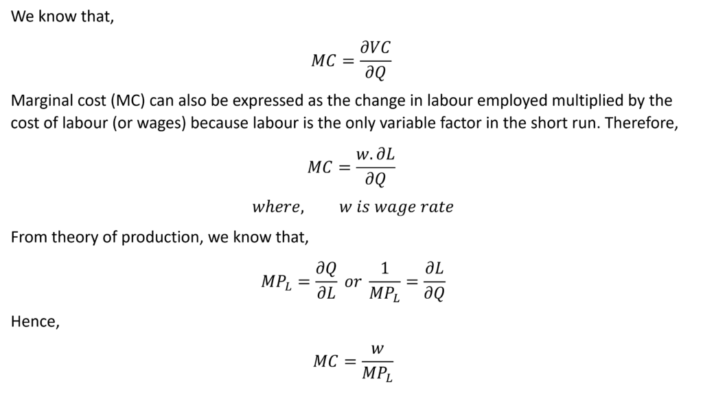
This means that when only one factor is variable (labour in the short run), marginal cost is the price of input (wages for labour) divided by its marginal product (MPL).
When marginal product of labour (MPL) is low, marginal cost will be high. The marginal cost will be low when the marginal product of labour (MPL) is high. If diminishing marginal returns exist, the marginal product of labour will decrease with an increase in output. As a result, marginal costs will increase as output increases.
cost curves in the short run
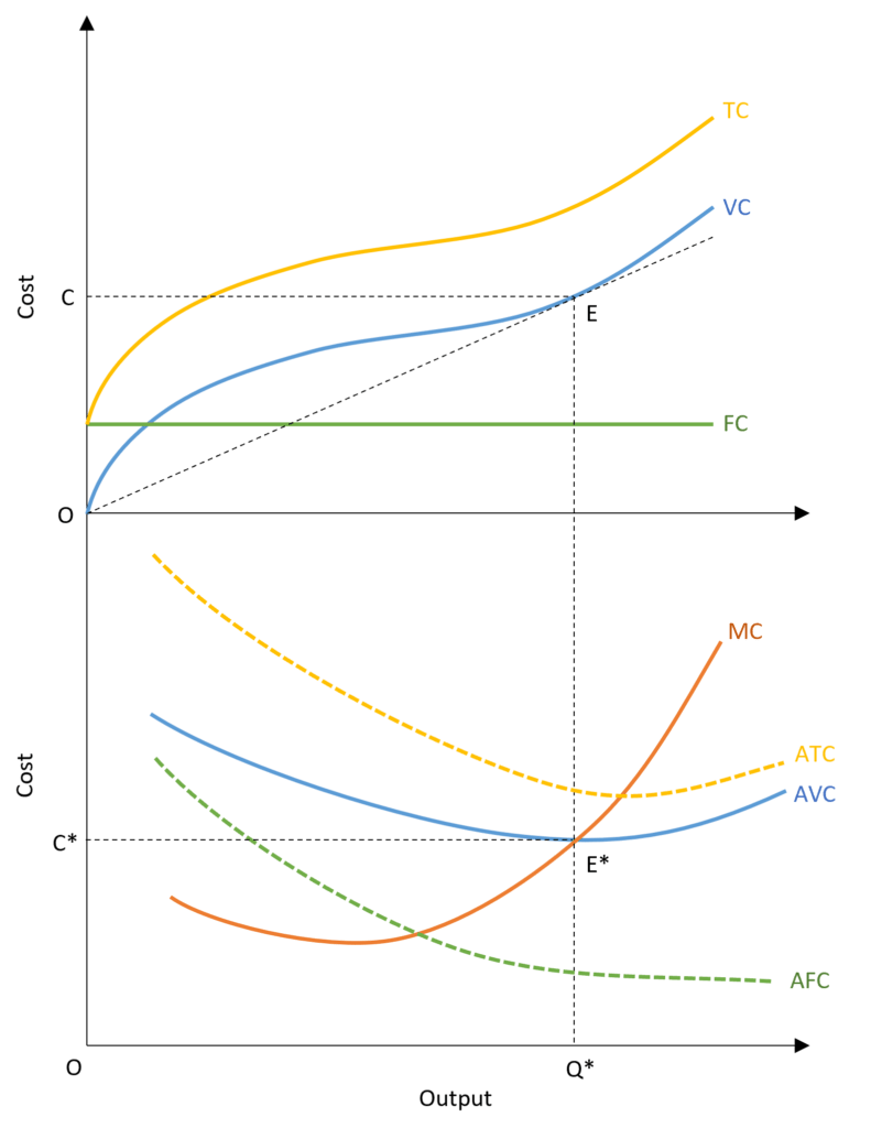
In the diagram, the fixed cost curve (FC) is parallel to the x-axis because it does not vary with output. The variable cost curve (VC) is zero when there is no output produced and goes on increasing with the rise in output. The total cost curve (TC) is the vertical summation of fixed and variable costs. Hence, the distance between the total cost curve (TC) and variable cost curve (VC) is always the same and is equal to the fixed costs.
The lower part of the diagram shows marginal and average cost curves. The average fixed cost curve (AFC) is declining with output because fixed costs remain the same whereas the output increases. When the output is one unit, AFC is equal to the FC and it goes on declining as output increases.
Relationship between Marginal and Average Cost curves
When marginal cost (MC) is less than average costs, the average cost curves are falling or downward sloping. When marginal cost (MC) is greater than average costs, the average cost curves are rising or upward sloping. Hence, the MC or marginal cost curve cuts the average cost curves from below at their minimum points. At the point where MC=AVC, the AVC is at its minimum and the MC cuts it from below. Similarly, at the point where MC=ATC, the ATC is at its minimum and MC cuts it from below.
This relationship is similar to that of average and marginal products discusses in production theory. When MC < AVC (or ATC), the average cost will decrease. This happens because the increment in cost with an extra unit of output is lower than the average. On the opposite end when MC > AVC (or ATC), the extra cost of producing one more unit of output is higher than the average cost, thus, the average cost will rise.
AFC, AVC and ATC
Because AFC goes on decreasing, the distance between AVC and ATC also decreases with output. They keep moving closer as output increases. The AVC reaches its minimum point before or at a lower output than the ATC. This happens because ATC is always greater than AVC (ATC = AFC + AVC) and the marginal costs are rising. As a result, the minimum point of ATC is always at a larger output as compared to the minimum point of AVC.
The line OE in the upper part of the diagram shows the average variable cost (AVC) at the output of Q*. This line is also tangent to the VC or variable cost curve and shows the marginal cost. Hence, this is the point where MC = AVC or the point where marginal cost and average variable cost curves intersect.
Econometrics Tutorials with Certificates

This website contains affiliate links. When you make a purchase through these links, we may earn a commission at no additional cost to you.