The ordinal utility analysis involves indifference curves and budget lines to determine consumer choice. A consumer will choose the quantity of a commodity that maximizes utility, given the budget constraint. This approach can also be used to derive the individual demand curve, Income-consumption and Engel curves of a consumer for the given commodity.
Econometrics Tutorials with Certificates

Changes in price of commodity: deriving the demand curve
Let us consider the example of two goods- shirts and muffins. Initially, the consumer is at equilibrium at point B which lies on I1, where:
MRS = P1/Pshirts
The price of muffins is P1 and the consumer will purchase B1 quantity of muffins and A1 quantity of shirts at this point.
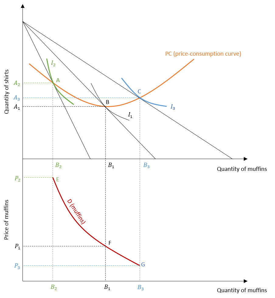
Suppose, the price of muffins increases. Then, the budget line will rotate to the left because the consumer can buy less quantity of muffins with a rise in price. Here, the consumer will be at a new equilibrium point A. At point A, another indifference curve I2 will be tangent to the new budget line. Here, MRS is equal to the ratio of new prices which includes a higher price of muffins.
MRS = P2/Pshirts
Additionally, the consumer will be at a lower utility because I2 is associated with lower utility than I1. The consumer will buy less quantity of muffins B2 at this higher price P2.
On the other hand, a fall in the price of muffins will rotate the budget line to the right. The consumer can buy more muffins because of a fall in price. The equilibrium point will shift to C, where the consumer will buy a higher quantity of muffins, equal to B3. This new indifference curve I3 gives higher utility to the consumer. At C,
MRS = P3/Pshirts
Note: the quantity of shirts may increase or decrease depending on the equilibrium points. But, the quantity of muffins will increase with a fall in price and decrease with a rise in the price of muffins.
Demand curve and Price-Consumption Curve
The lower part of the figure shows the individual demand curve of the consumer for muffins. It illustrates the different quantities of muffins associated with different prices. At a higher price, demand for muffins is lower and it increases with a fall in price. At P2 price, demand for muffins is low at B2. As the price keeps falling to P1 and further to P3, demand for muffins keeps increasing to B1 and further to B3.
The price consumption curve shows all possible utility-maximizing combinations of two goods (shirts and muffins), in response to changes in the price of muffins. We observed that as the price of muffins changes, the equilibrium points also change. The figure shows three different utility-maximizing points (A, B and C) at three different prices of muffins (P1, P2 and P3). The price consumption curve is created by tracing all these utility-maximizing points, at all possible prices of muffins.
Features of Demand curve and Price-Consumption curve
- The level of utility changes with movement along the curves. As the price of muffins falls, the consumer moves along the demand curve and price consumption curve and the level of utility goes on increasing. This happens because the consumer is moving to a higher indifference curve. Hence, the lower the price of muffins, the higher the level of utility associated with that price.
- The consumer maximizes his or her utility at every point on the demand curve and the price consumption curve. Equilibrium is attained through the equivalence of MRS with the ratio of prices. The equilibrium point changes with a change in price, but, it is always a utility-maximizing point. Furthermore, the falling price of muffins also means that MRS is diminishing as the price ratio falls. It makes sense because the marginal utility of muffins falls as the consumer keeps purchasing more of them.
Changes in income of consumer: deriving Income-consumption and Engel curves
A change in the income of consumers leads to a shift in the budget line. As income increases, the budget line shifts parallel to the right because consumer can buy more of both shirts and muffins with higher income. Conversely, there is a parallel shift to the left in the budget line with a decrease in income as the quantity consumed of both goods will fall.
Initially, the consumer maximizes utility and is at equilibrium at point B on I1, where:
MRS = P1/Pshirts
At this income level, the consumer will purchase A1 and B1 quantities of shirts and muffins respectively.
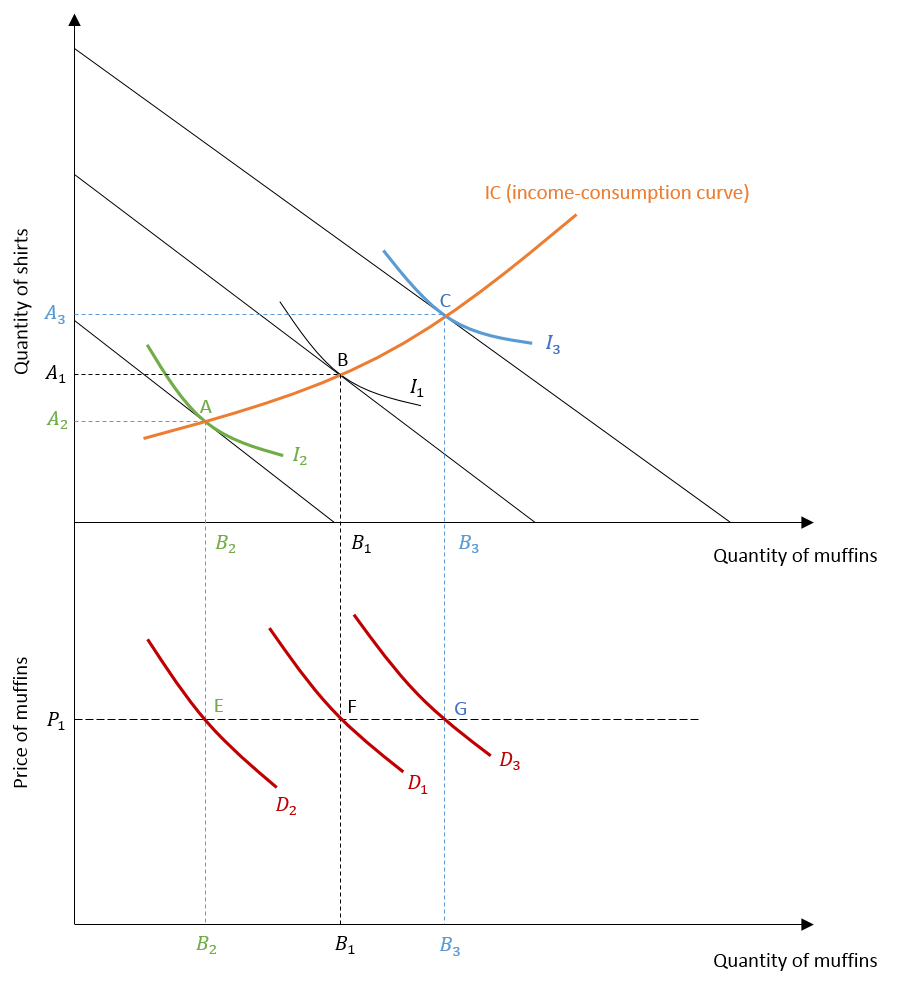
Suppose, the income of the consumer falls. The budget line will shift to the left and a new equilibrium level is attained at point A, which maximizes utility at that lower income level. Because the price of both goods remains constant, the shift in the budget line is parallel. The quantity of both goods falls to A2 and B2.
On the other hand, an increase in income leads to a parallel shift in the budget line to the right and utility is maximized at point C, where a higher quantity of both commodities is purchased because of higher income.
Demand curve and Income-Consumption curve
In the case of price changes, we observed a movement along the demand curve. However, for changes in income, the demand curve will shift to the right with an increase in income. It will shift to the left with a fall in income. As income falls, we can observe a leftward shift in the demand curve from D1 to D2.
On the other hand, the demand curve shifts to D3 with rise in income level. Moreover, the higher the income elasticity, the bigger will be the shift in the demand curve. This happens because a rise in income will lead to a higher increase in quantity demanded when income elasticity is high for the goods concerned.
These demand curves represent different income levels. With changes in price, these demand curves will be traced out at those particular levels of income. For instance, demand curve D3 will trace out the effects of changes in the price of muffins at that income level. Since we are holding prices constant, we observe only points E, F and G on the demand curves D1, D2 and D3 respectively, which correspond to separate levels of income.
The income consumption curve traces out all possible utility-maximizing combinations of two goods (shirts and muffins) with respect to all possible levels of income. It is an upward sloping curve because consumption of both goods increases with an increase in income level. Similar to points A, B and C, this curve represents all points of equilibrium associated with different income levels. With movement along the income consumption curve, consumer moves to higher levels of utility as income rises.
Income-consumption and Engel Curves
The Engel curve shows the quantity demanded of a commodity in response to changes in the income level of a consumer. In other words, they represent the relationship between quantity demanded and income. Engel curve for any commodity can be derived from the income consumption curve.
The income consumption curve depicts the utility-maximizing combinations of two goods at different levels of income. In the earlier example, we examined the income consumption curve of shirts and muffins. In that case, the effects of changes in income were depicted by shifts in the budget line.
Deriving the Engel curve
To derive the Engel curve of muffins, the quantity demanded of muffins is represented as a function of income. That is, we plot income levels on the y-axis instead of the quantity of shirts. Since we already know the different quantities of muffins at different income levels from the income consumption curve, we can easily derive the Engel curve by plotting the quantity of muffins against the income level.
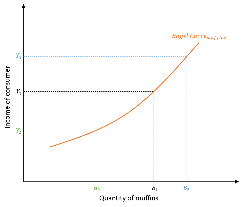
The quantities B1, B2 and B3 in the diagram are the same as the quantity of muffins shown earlier in the income consumption curve. The difference lies on the y-axis. It shows the corresponding income levels Y1, Y2 and Y3 respectively instead of the quantity of shirts. These income levels were depicted as shifts in budget lines while constructing the income consumption curve.
With a fall in income from Y1 to Y2, the budget line shifts to the left and the quantity of muffins falls to B2. The budget line shifts to the right with rise in income from Y1 to Y3 and quantity demanded of muffins increases to B3. This same relationship is shown in the Engel curve. The quantity of muffins increases with an increase in income and decreases with a fall in income.
Income elasticity: Here, the Engel curve shows positive income elasticity of demand because quantity of muffins is increasing with the increase in income. There is a positive relationship between the two and the curve is upward sloping. This also shows that muffins are normal goods as they have a positive income elasticity of demand.
Special case of Inferior Goods: Income-consumption and Engel curves
Inferior goods can be defined as goods having a negative income elasticity. The quantity demanded of these goods falls with a rise in income. Hence, there is a negative relationship between quantity demanded and income. Let us examine the income consumption curve of an inferior good and the resultant Engel curve:
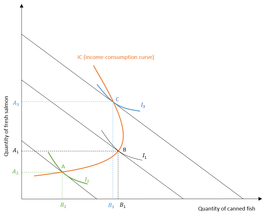
In this example, canned fish is an inferior good. At low levels of income, the quantity demanded increases with a rise in income and canned fish is a normal good. However, as the income keeps rising, the consumer prefers fresh salmon over canned fish. Therefore, the quantity demanded of canned fish starts to fall with an increase in income. This happens because it is an inferior good for the consumer at a high-income level.
On the other hand, fresh salmon is a normal good and its quantity demanded keeps rising with an increase in income. As a result, the income consumption curve bends backwards at high-income levels due to decreased consumption of the inferior good (canned fish).
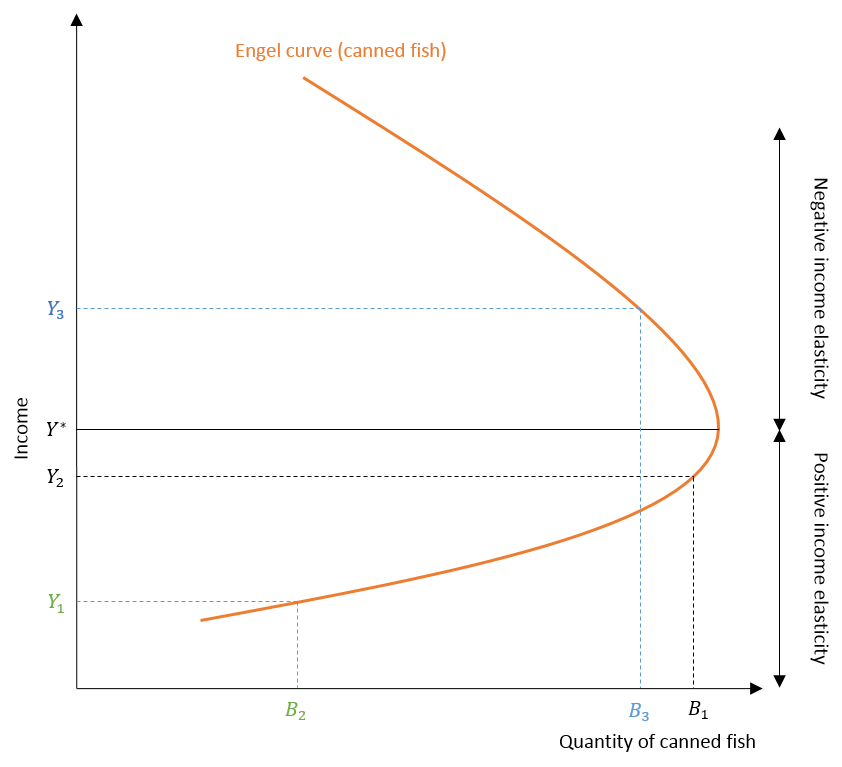
Similar to the income consumption curve, the Engel curve associated with canned fish is backward bending because it is an inferior good. Initially, the Engel curve slopes upward at low-income levels when canned fish is a normal good. As income increases above Y*, the Engel curve bends backwards because canned fish becomes an inferior good.
Since canned fish is a normal good below Y*, income elasticity is positive. Beyond this Y* level of income, the income elasticity of demand becomes negative for canned fish. Moreover, the quantity demanded of fresh salmon keeps increasing with income because it is a normal good at all income levels of the consumer. Hence, its income elasticity is always positive.
Econometrics Tutorials with Certificates

This website contains affiliate links. When you make a purchase through these links, we may earn a commission at no additional cost to you.