The Sargan Test of Overidentifying Restrictions is applied to check the validity of the instruments used in simultaneous equation models. As the name suggests, it is applicable to overidentified model equations.
Overidentification implies that the number of endogenous regressors is less than the number of instruments used in the given equation. It can be easily determined using Order and Rank conditions of Identification. Identification is one of the essential and initial steps in estimating simultaneous equation models. Furthermore, if an equation or model is overidentified, tests of overidentifying restrictions must be applied to check the validity of instruments. When an equation or model is just or exactly-identified, such tests are not applicable.


Specification of the Model
To illustrate the procedure of the test, let us consider an overidentified simultaneous equation model. We will use the same model that we estimated in Two-Stage Least Squares (2SLS) Estimation.
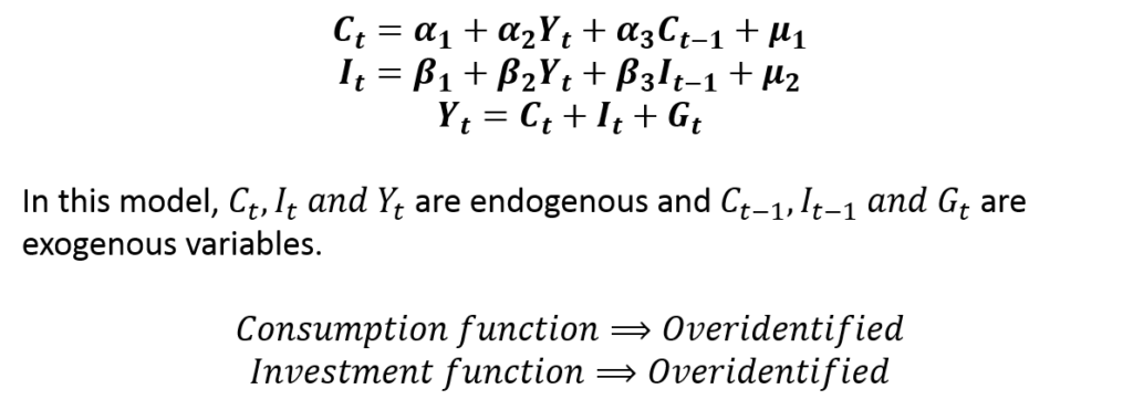
This model can be estimated using 2SLS because both the consumption and investment equations are overidentified. Moreover, the results of both equations are available in Two-Stage Least Squares (2SLS) Estimation.
Since the equations are overidentified, we must apply the Test of Overidentifying Restrictions to check whether the instruments are valid. This will also show us if any of the equations is misspecified. We will illustrate the Sargan Test here:
Procedure of the Sargan test of overidentifying restrictions
STEP 1: Estimate the simultaneous equation model.
The consumption and investment functions have to be estimated using any of the suitable methods. In our example, we used the 2SLS approach as it is applicable to overidentified models. The results of the model are available in Two-Stage Least Squares (2SLS) Estimation.
We do not need to present the results of the model here. We will focus on the application of the Sargan Test.
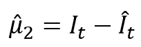
STEP 2: Obtain the residuals from the equations of the simultaneous equation model.
In our example, we will focus on the investment function because it provides us with interesting results. The consumption equation was observed to be correctly specified after applying the test. But, the investment function is misspecified as the results of the Sargan Test will reveal. Hence, we will move forward with the analysis of the investment equation only for illustration.
Therefore, we will predict the residuals from the investment equation after estimation using 2SLS.
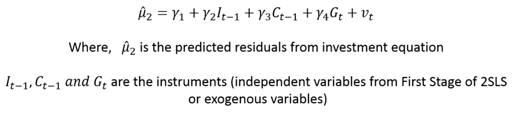
STEP 3: Regress the residuals on all the instruments used in the equation.
The instruments are all the exogenous variables used in the First Stage of 2SLS to estimate the Endogenous Regressor. In our example, Income (Yt) is the endogenous regressor whose predicted value is used as an instrumental variable in the Second Stage. All the instruments include the variables that were used to predict Income in the First Stage. In our example, these instruments include all the exogenous variables (Ct-1, It-1 and Gt).
STEP 4: Finally, apply Chi-square Test.
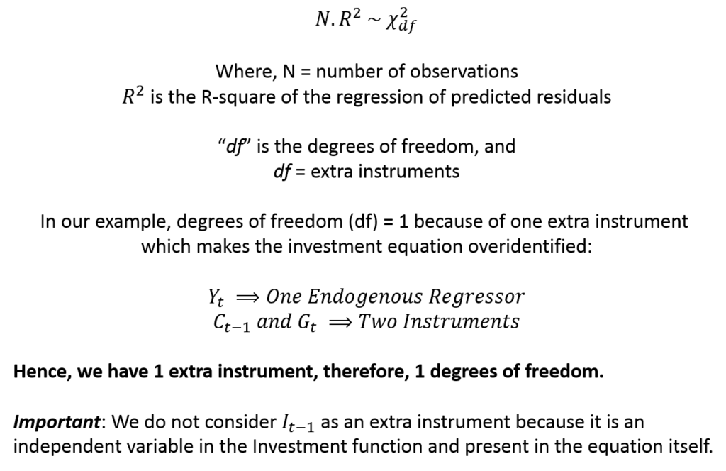
Hypothesis of the test
The Chi-square value can be used to test the hypothesis of whether the instruments are valid. Since these instruments are excluded from the investment equation itself, it also tells us whether they have been correctly excluded.
H0: the instruments are valid and correctly excluded from the investment function.
HA: the instruments are invalid.
If the Chi-square test gives us a significant p-value, we reject the null hypothesis and conclude that the instruments are invalid. Otherwise, we do not reject the null hypothesis.
Application and interpretation in practice
The test results can be easily computed using statistical software packages. That is, we do not need to carry out the test manually.
In our example, we applied the Sargan Test of Overidentifying restrictions to consumption and investment functions. The test revealed that the consumption function has been correctly specified and the instruments are valid.
However, the results of the investment function tell a different story. Let us look at the results:
| Sargan Test | |
| Chi2 (1) = 50.6986 | p = 0.000 |
As noted before, the degree of freedom (df) is 1 because we have one extra instrument that makes the model overidentified. We reject the null hypothesis because the p-value shows significant results. Hence, we conclude that the instruments used in the investment function are invalid.
Important: This result of the Sargan Test can be an indicator that the instruments may be incorrectly excluded from the investment function. That is, we may have used Ct-1 or Gt incorrectly as instruments. Instead, these variables may belong in the investment function itself. In addition to explaining the endogenous regressor (Yt), these variables may also be significantly affecting investment directly. This implies that we should try including these variables in the investment equations alongside It-1.
The investment equation, therefore, is misspecified. This was expected because we applied a very simple model to explain complicated economic relationships between income, consumption and investment. We may have to try different specifications by including Ct-1 or Gt in the investment function. We might need to get additional data on important variables such as the rate of interest, which may significantly affect investment.
Econometrics Tutorials with Certificates


This website contains affiliate links. When you make a purchase through these links, we may earn a commission at no additional cost to you.