The Vector Error Correction Mechanism (VECM) is estimated in the presence of cointegration among the system of variables. It allows us to estimate short-run as well as long-run coefficients. Using VECM estimation, we can analyze long-run equilibrium relationships among variables and short-run deviations from that equilibrium. Moreover, the adjustment coefficients show us how the short-run deviations or disequilibrium are corrected.
Here, we will discuss the procedure to estimate a VECM model and the interpretation of its results. To keep all the analysis simple, we will use a two-variable (Xt and Yt) dataset to illustrate all the steps of estimation and interpretation. To learn more about the theory associated with VECM, read the Vector Error Correction (VECM): Theory post.

The Procedure of VECM estimation
Step 1: Choose the number of lags
As discussed in Vector Error Correction (VECM): Theory post, every VECM model also has an underlying VAR model. The choice of the appropriate number of lags is essential in VAR and VECM models. Incorrect lag length specification can lead to specification errors, and inaccurate results and may cause the problem of autocorrelation.
Moreover, the number of lags in VECM is always one less than the underlying VAR model. If the underlying VAR model has 3 lags, its VECM will have 2 lags of differences. This is because the underlying VAR is specified for original variables, whereas, the VECM has variables in their first difference form.
To choose the appropriate number of lags for underlying VAR, various Information Criteria can be used. The VECM will automatically have one less lag in differences. Akaike’s Information Criteria (AIC), Schwarz or Bayesian Information Criteria (SIC or BIC) and Hannan-Quinn Information Criteria (HQIC) are often used for this purpose. The post on Information Criteria and Model Selection discusses these in more detail.
Information Criteria and VECM lag-length
| VAR Lag order | AIC | SIC | HQIC |
| 0 | -0.568399 | -0.514976 | -0.546805 |
| 1 | -3.95166 | -3.79139 | -3.88688 |
| 2 | -3.88178 | -3.61466 | -3.77381 |
| 3 | -3.93802 | -3.56405 | -3.78686 |
| 4 | -3.93508 | -3.45426 | -3.74072 |
All the Information Criteria have a minimum value for lag order 1. This implies that the underlying VAR model with lag 1, therefore, a VECM with 0 lagged differences or without any lagged differences is a good starting point.
Important: it is essential to ensure that the VECM doesn’t suffer from autocorrelation. In this example, it was observed that a VECM without lagged differences (underlying VAR with 1 lag) suffered from autocorrelation. Hence, more lags need to be included in the VECM to eliminate autocorrelation. The use of 3 lags in VECM, that is, 4 lags in the underlying VAR model gets rid of the problem of autocorrelation in this example. See the post on the VAR-VECM Goodness of fit to learn more about the autocorrelation tests and other methods to check the fit of VECM models.
Hence, we will proceed with 4 lags in the underlying VAR model or 3 lagged differences in VECM to eliminate autocorrelation in the model.
Step 2: Determine trend specification for Johansen’s Test of Cointegration and VECM
The VECM framework by Johansen allows five different types of trend specifications:
- Unrestricted Trend: quadratic trend in levels and trend stationary cointegrating relationship.
- Restricted Trend: linear trend in levels and trend stationary cointegrating relationship.
- Unrestricted Constant: linear trend in levels and the cointegrating relationship may be stationary around a constant non-zero mean.
- Restricted Constant: no linear trend in levels and the cointegrating relationship may be stationary around a constant non-zero mean.
- No trend: no linear trend and the cointegrating relationship is stationary around zero mean.
To get some intuition on the behaviour and trends of the variables, we can plot the variables with time on the x-axis.
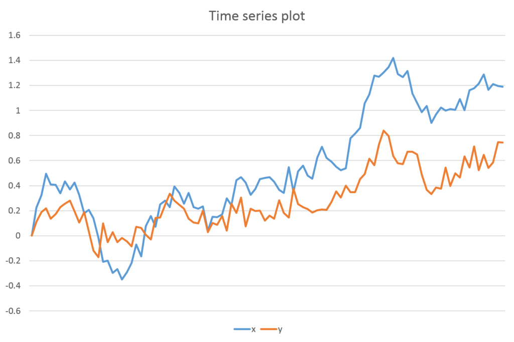
The variables “x” and “y” seem to be moving upward, thus, eliminating the “No trend” specification. The trend is not quadratic in nature implying that the “Unrestricted Trend” option is not applicable. Because we may have a linear trend or drift in levels, “Restricted Constant”, “Unrestricted Constant” or “Restricted Trend” specifications may be used. If the cointegrating equation from the estimated VECM shows a trend, then we must use “Restricted Trend”. If the cointegrating equation is stationary around a constant mean (without trend) and there is a linear deterministic trend in levels, it means that we can use the “Unrestricted Constant” specification.
Hence, it is advisable to try different VECM specifications and compare the results. Based on the stationarity of the cointegrating equations, we can decide which specification to use for the final analysis. Hence, “Restricted Trend” may be used if the cointegrating equation is trend stationary.
In this example, we will only present the results for the “Unrestricted Constant” specification for illustration purposes. In practice, you may have to apply Johansen’s Test of Cointegration and the VECM model to different specifications before deciding on the correct one.
Step 3: Apply Johansen’s Test of Cointegration
Johansen’s Test of Cointegration is used to determine the number of cointegrating vectors or cointegrating relationships (r). The VECM model is used if the cointegrating vectors are greater than 0 and less than the number of variables in the model (K).
0 < r < K; apply VECM
In our example (where K = 2), application of VECM is appropriate if r = 1 because it satisfies the above condition 0 < r < K (i.e. 0 < 1 < 2). In practice, we should apply Johansen’s Test of Cointegration for other specifications as well. Although we may have some theoretical indications about the variables, we have no definite information about the stationarity of the cointegrating equations.
Here, we will present the results of the “Unrestricted Constant” specification of VECM only. The test can be performed using either the Trace statistic or the Maximum Eigenvalue statistic to test the following hypothesis:
Trace and Maximum Eigenvalue statistics
| Cointegrating vectors or rank (r) | Trace Statistic | Maximum eigenvalue statitic |
| 0 | H0: no cointegration and, HA: at least 1 cointegrating vector | H0: no cointegration and, HA: 1 cointegrating vector |
| 1 | H0: 1 cointegrating vector HA: at least 2 cointegrating vectors | H0: 1 cointegrating vector HA: 2 cointegrating vectors |
| 2 | No need to test further because rank = 2 if above H0 is rejected for rank <= 1 | No need to test further because rank = 2 if above H0 is rejected for rank = 1 |
The above hypothesis are tested sequentially in Johansen’s Test. The results of the test for our example with Unrestricted Constant are:
| Cointegrating vectors or rank (r) | Trace statistic | Critical value at 5% | Max statistic | Critical value at 5% |
| 0 | 20.2099 | 15.41 | 19.5034 | 14.07 |
| 1 | 0.7064 | 3.76 | 0.7064 | 3.76 |
| 2 |
We start from rank 0 and reject the null hypothesis if the statistic is greater than the critical value. In such a case, we move on to the next rank in sequence. The null hypothesis of no cointegration can be rejected using both the trace and max statistic. The test statistics are greater than the critical values.
Next, move on to test for rank 1. We conclude that there is 1 cointegrating vector because we cannot reject the null hypothesis for both tests. The null hypothesis for trace statistic states that there is no more than 1 cointegrating vector. We cannot reject this null hypothesis because the test statistic is less than the critical value. Similarly, we cannot reject the null hypothesis of 1 cointegrating vector using the max statistic.
Hence, we conclude that there exists one cointegrating or long-run relationship.
Step 4: VECM Estimation
Now that we know the number of cointegrating vectors and the number of lags to be used, we can estimate the VECM model. After estimation, we can obtain the cointegrating equations and decide which specification is more suitable.
Important: the choice of trend specification can also be made based on the forecasting power of the models. We can choose the model which gives better forecasts with low forecast error. The choice may depend on the purpose of the analysis.
For our example, we will use the “Unrestricted Constant” specification for the estimation and interpretation of the results.
Interpretation of VECM
In our example, the results of the VECM (unrestricted constant) with 4 lags in underlying VAR (or 3 lagged differences in VECM) and 1 cointegrating relationship are:
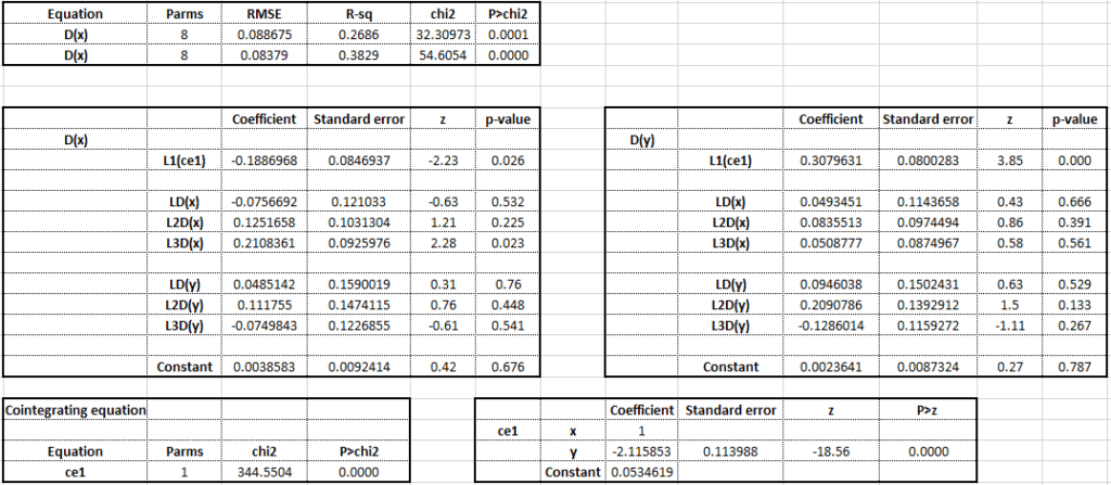
These results contain short-run impacts, short-run adjustment coefficients as well as the long-run cointegrating relationship between “x” and “y”. The two tables in the middle show short-run coefficients for both the equations of the VECM. These include short-run adjustment coefficients and short-run impact coefficients of all the lagged differences.
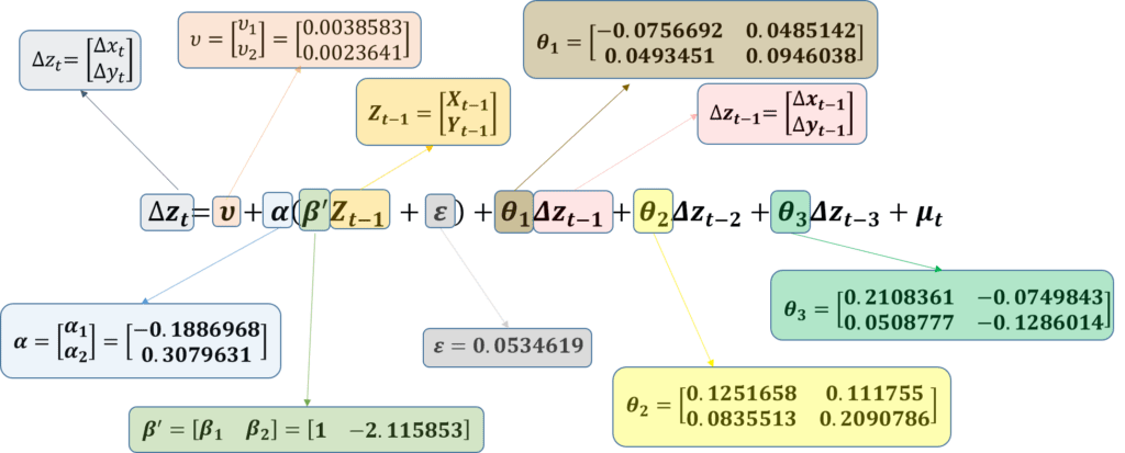
Cointegrating vector
The cointegrating vector or long-run coefficients are shown in the bottom-right table.

This cointegrating vector represents the long-run equilibrium relationship between x and y. In the short run, however, there are some deviations or errors and the variables do not stay at their long-run equilibrium.
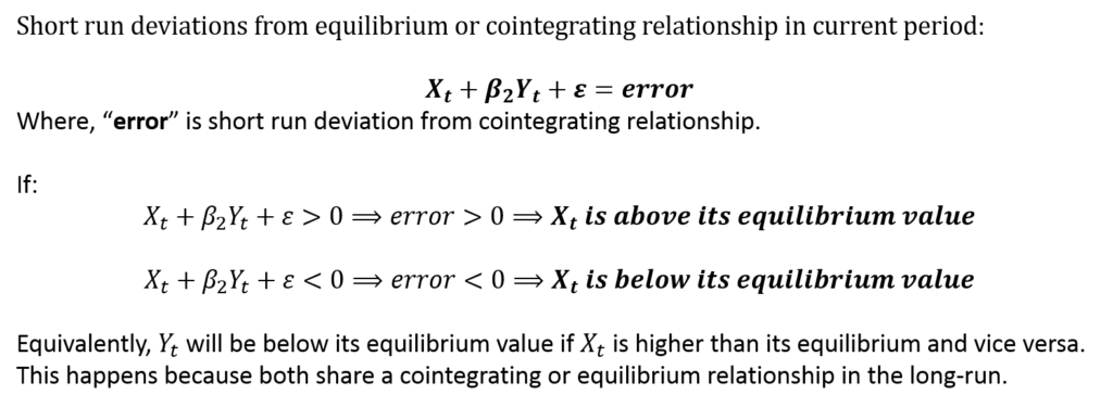
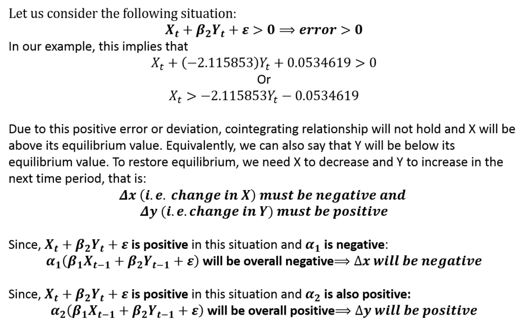
If this error is positive, it means that xt will be above its long-run equilibrium value. That is, the value of “x” and “y” will deviate up or down from its cointegrating/equilibrium relationship according to this error. The convergence back to equilibrium or correction in short-run error/deviations is determined by the adjustment coefficients.
Adjustment coefficients and their signs
The adjustment coefficients are shown in the vector “alpha”. In the table, these coefficients are present in each equation as “L1(ce1)“. These coefficients show the speed of convergence towards long-run equilibrium. In the short run, the variables can deviate from long-run equilibrium or cointegration relationships. The adjustment coefficients depict how these deviations will be corrected.
For convergence, the signs of these adjustment coefficients must be correct. Otherwise, the deviations will explode and long-run equilibrium will not be restored. This means that our VECM is not correctly specified.
In our example, the adjustment coefficient for the first equation must be negative and significant. This will ensure convergence toward long-run equilibrium.
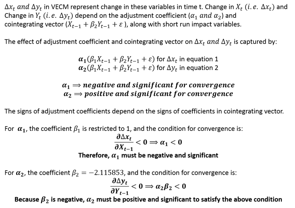
In case X is above its equilibrium value, a negative adjustment coefficient will ensure that the value of X will fall in the next time period. Similarly, if the short turn deviation/error is negative and X is below its equilibrium value, a negative adjustment coefficient will ensure that the overall effect is positive. The value of x will increase in the next time period. Hence, convergence towards equilibrium will occur automatically.
The same logic applies to Y and the change in Y. Its adjustment coefficient must be positive and significant to achieve convergence. This happens because the associated coefficient with Y is negative in cointegrating equations. Hence, the adjustment coefficient must be positive for the overall effect to be negative. Let us take a look at an example of how it will work in practice:
Identification Restrictions in VECM
The long-run relationship or cointegrating vector is shown in the bottom-right table. Being a simultaneous equation model, we must ensure that the model is identified. To make a VECM model identified, some restrictions must be imposed. In our example, the coefficient of x = 1 restriction is imposed on the cointegrating vector. This is also known as Johansen Normalization.
In general, r2 number of restrictions must be introduced in a VECM model for identification (r = number of cointegrating relationships). Hence, if the model has 2 cointegrating relationships, we must introduce at least 4 restrictions. In our example, VECM has 1 cointegrating relationship. Therefore, 1 restriction is enough because r2 = 12 = 1.
Further analysis after vECM estimation
Before proceeding with further analysis and forecasting, researchers must ensure that the VECM model is a good fit. The Goodness of fit statistics for VECM and VAR models include stability tests, autocorrelation tests and normality of error terms. These texts are discussed separately in VAR and VECM Goodness of fit. The fit of the model must be checked before proceeding with further analysis.
Usually, the other coefficients of VAR and VECM do not have any meaningful interpretations directly. Instead, these models are preferred for forecasting purposes. Another important use of these models is the Impulse Response Functions (IRFs). The IRFs and OIRFs give a lot of useful information on the behaviour of variables in the models and their effects on each other. The analysis of IRFs is discussed in detail in Impulse Response Functions after VAR and VECM.
Econometrics Tutorials with Certificates


This website contains affiliate links. When you make a purchase through these links, we may earn a commission at no additional cost to you.
Thanks for this. The detailed visual breakdown of the VECM equation is very useful.
You’re welcome
Thank you for sharing. But I have one question on IRFs of VECM. Is it mandatory to present confidence bands on VECM’s IRFs? Some of them are not significant, can they still be used?
The confidence bands are important because they show how certain you can be about the effects of impulses. If the zero value lies within the confidence bands, your IRFs might be zero or the effect seen in IRFs might be due to chance. You can’t be certain whether the effect is truly significantly different from zero. So, it is advisable not to ignore the confidence bands and you should present them with the IRFs.
However, you might want to look deeper and consider why you have insignificant IRFs. Is it possible that the effect might actually be zero and the shocks don’t effect other variables in reality? It could be due to your sample as well, maybe you have insufficient data to capture all the effects. Similarly, you should also look into the specification of your VECM. Are you missing some variables or is the specification of the model correct?
Hello,
May I cite the information in this website?
Yes, please go ahead. You can use the following guide to cite the information:
Rehal, Viren. “Page Title.” Spur Economics, URL of the page. Accessed Day Month Year.
Thank you