Cardinal and ordinal utility analysis assume that all the variables, such as prices and income, are known with certainty. However, this is not the case in reality. Consumers have to make decisions based on uncertain outcomes and variables. For instance, future prices and income can never be known with certainty and there is a level of risk involved while making some consumption or investment decisions. As a result, consumer choice under uncertainty and risk must be carefully examined.
Consumers make major consumption and investment decisions based on uncertain variables. For example, a student opts for an educational loan in expectation of paying back the loan with future income which is uncertain. Investment decisions by firms involve uncertain outcomes because it is impossible to know whether the investment will be a success or a failure. Hence, decisions or choices are often made under uncertainty. Such decisions involve the role of probability of different outcomes, expectations of the future and risk.
Econometrics Tutorials with Certificates

Probability and Expected Value
Role of probability
Probability refers to the likelihood that a given outcome will occur. The number of outcomes may vary depending on the event. For instance, a flip of a coin generally has two outcomes- heads or tail. If it is a fair coin, then the probability or likelihood of getting heads is 0.5 and the probability of tails is 0.5. Similarly, a roll of a fair dice has six different outcomes, each with the same probability of 1/6 (0.167). It is important to note that the sum of probabilities of all outcomes is always one.
For instance, the outcomes of an investment decision may be two- success or failure, with different probabilities. The probability assigned to each outcome (success or failure) may be based on different aspects. The probability of success of investment may be decided on the basis of previous similar investments and their success rate. If the previous similar investments had a 75% success rate, then, the firm or individual may conclude that the investment has a 0.75 probability of success and 0.25 probability of failure.
Sometimes, previous information is not available and probabilities associated with different outcomes have to be decided using other information. This may include information such as individual expertise of investor or market information. In many cases, probabilities are subjectively decided. That is, people have a different perspective of outcomes and their probabilities, leading to different choices by them.
Expected Value
The value or payoff associated with each outcome and the probability of those outcomes is used to determine the expected value. The expected value can be estimated as follows:
Expected value = P1X1 + P2X2 + … + PiXi
where, P refers to probabilities (0 < P < 1 and P1 + P2 + … + Pi = 1), X refers to value of outcomes and i is total number of outcomes.
Therefore, the expected value is the weighted average of the value of outcomes. The weights are determined by the probability of each outcome.
Let us consider an investment decision that has a payoff or value of $50 for success outcome and a payoff of $10 if it’s a failure. Suppose, the probability of success is determined by the investor to be 0.75. The expected value of this investment will be:
Expected value = PSXS + PfXf
Where, PS is the probability of success and XS is the payoff from success, Pf is the probability of failure and Xf is the payoff from failure.
Expected value = 0.75(50) + 0.25(10)
Hence, Expected value = 40
We can say that the expected value of the investment is $40.
Risk
The risk associated with any decision is the standard deviation of outcome values from the expected value. Higher the standard deviation, the higher the risk accompanied by the decision.
In the previous example, we estimated the expected value to be $40 for investment. We also know the probabilities of success and failure of the investment, along with the outcome values. This information can be used to estimate standard deviation or Risk:
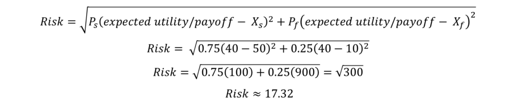
Suppose, there is another investment opportunity available with the same expected value of $40. But, the probability of success and outcome values are different for this investment. Let the probability of success be 0.5 with an outcome value of $45 and the outcome value or payoff of failure be $35. Then, the expected value will be calculated in the same manner as before:
Expected value = PSXS + PfXf
Expected value = 0.5(45) + 0.5(35)
Hence, Expected value = 40
Therefore, the expected value of the investment is the same for both investment opportunities. However, the risk involved is different. Let us estimate the risk of this new investment:
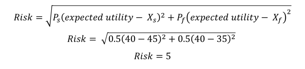
Hence, we can observe that the risk involved in the new investment opportunity is much less as compared to the previous investment. This happens because the variability of outcome values is low in the case of new investment. The new investment has a $35 payoff even in failure as compared to the $10 value of failure outcome from earlier investment.
Risk Preference and Choice under Uncertainty
In the example above, one investment has a higher payoff of $50 in case of success, but, it comes with high risk. The other investment involves less risk, but, a lower payoff of $45 with success. The actual decision or choice between the two investments will depend on the risk preference of the investor. If the investor is risk-averse, he or she will choose the investment with lower risk because the expected payoff is the same for both investments. On the other hand, a risk-taker will prefer the investment with a higher payoff of $50 and take on a high-risk investment.
Hence, the decision or choice under uncertainty is determined by the preference toward risk. Risk-averse consumers prefer lower risk and risk-takers prefer higher payoffs even in the presence of high risk. This phenomenon is easily applicable to consumer choices as well, where the payoff is in terms of utility. Let us look at how risk preference will affect utility and consumer choices.
Choice under Uncertainty: Risk Aversion
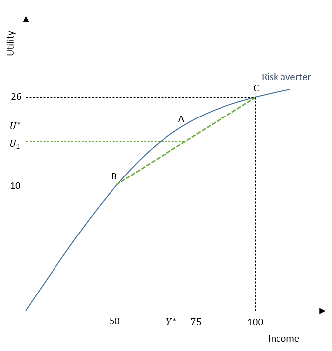
Suppose, a risk-averse individual receives a new job offer with the same expected income as the current job. But, the new job involves two outcomes. One outcome with the higher expected income is shown by C (where expected income is $100) and the other with the lower expected income is shown by B (where expected income is $50) with an equal probability of 0.5. The expected income of this new job is shown by point A and is equal to Y* ($75), which is also the income from the secure current job. Therefore, the expected income is the same for both jobs, but, the new job involves higher risk with two possible outcomes.
A risk-averse individual will choose to stay at the secure current job with no risk because it gives a higher utility of U*. On the other hand, the expected utility from the new job is U1. It is clearly lower than U* or the utility from the current job.
It can be observed that the utility curve of a risk-averse individual has a diminishing marginal utility of income. That is, as income increases, additional utility from rising income goes on decreasing. As a result, a risk-averse individual receives lower utility from a high-risk job. They will choose the low-risk option if the expected income is the same.
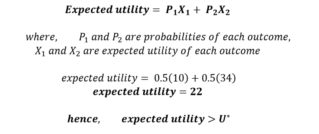
Calculating the Expected Utility
Let us assume that the individual can measure his or her utility and U* is equal to 20. Therefore, the utility from the current job is 20. In the case of the new job, the utility from the lower outcome is 10. Because of the diminishing marginal utility of income, the utility will increase at a decreasing rate. It reaches 20 at U*, but, it will be lower than 30 at the higher outcome (shown by point C) from the new job. This happens because of its diminishing nature. Let us assume that the expected utility is 26 at the higher outcome. Then, the expected utility from the new job can be estimated in the same manner as before:
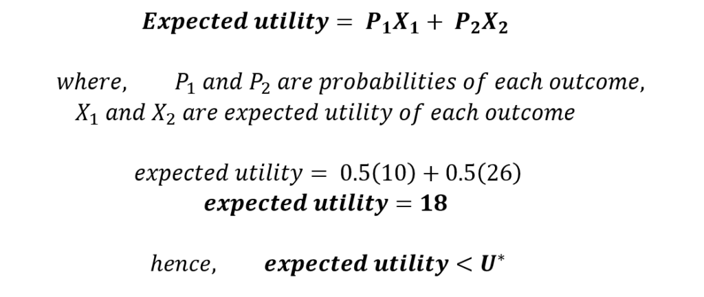
As a result, a risk-averse individual will choose to stay at their current job, which gives higher expected utility.
Choice under Uncertainty: Risk Taker
Let us consider the same example for a risk-taking individual and assume that he or she receives that same new job offer. The expected income from this new job is the same as the income from the current job and is equal to $75 (Y*). The new job involves the same high-risk outcomes with the probability of 0.5 for each outcome. Outcome at point
B shows a low expected income of $50 and the other outcome shows a high expected income of $100.
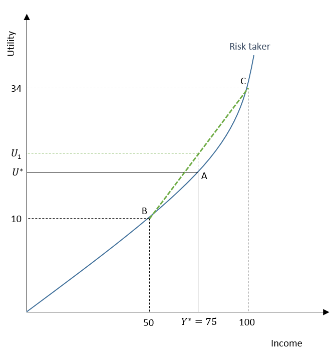
However, the choice of a risk-taker will be different from a risk-averse individual because of the higher expected utility of the new job. The expected utility of U1 from the new job is higher than the utility from the current job (U*).
This happens because a risk-taker has an increasing marginal utility of income. As seen from the curve, utility increases at an increasing rate with a rise in income. This results in a higher expected utility from the new job.
Because the risk-taker has an increasing marginal utility of income, the expected utility from a higher outcome (shown by C) will be greater than 30. Let us say, the expected utility is 34 for the higher outcome at C. We assume that the utility from the lower outcome is 10, similar to the previous case. Then, the expected utility for a risk-taker will be:
As a result, a risk-taker will choose to take the new job because the expected utility is higher than the utility of the current job (U* = 20). This happens because a risk-taker has an increasing marginal utility of income.
Choice under Uncertainty: Risk Neutral
If the current income and expected income from the new job are the same, a risk-neutral individual is indifferent between them. Considering the same example, the expected utility of the new job will be equal to the utility of the current job for a risk-neutral individual.
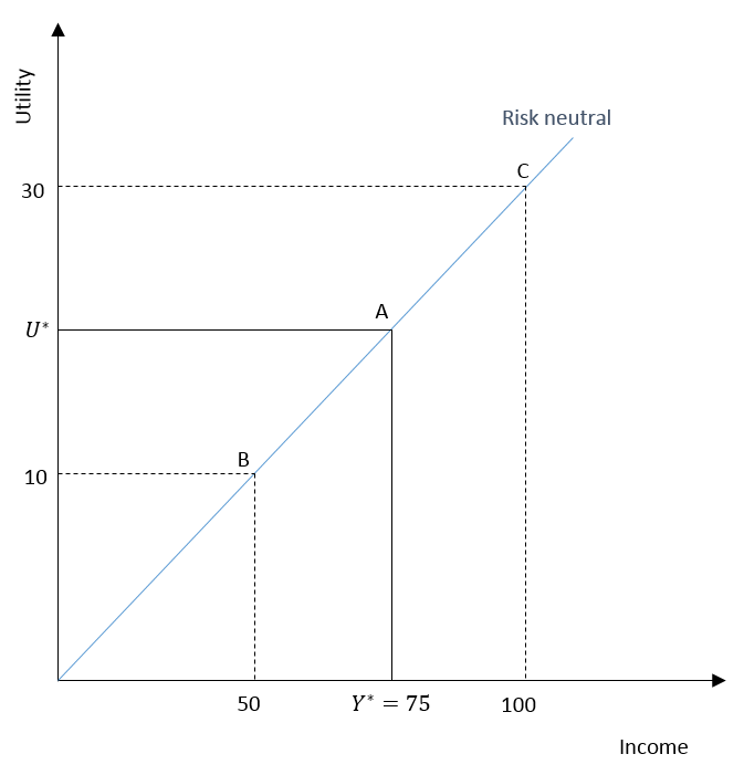
As observed in the diagram, a risk-neutral person has a constant marginal utility of income. That is, the marginal utility from additional income remains the same as the income keeps rising. As a result, expected utility and current utility are the same and the individual is indifferent between the two jobs.
Risk Premium
In our example, Risk premium can be defined as the amount of extra income a person would give up to become indifferent between the two jobs. For a risk-averter, it is the amount by which the income from the current job has to fall, to make the individual indifferent between the two jobs.
Let us continue with the earlier example of a risk-averse individual. We know that the expected utility was 18 from the new job, which was less than the current utility (U* = 20). In this case, the expected income from both jobs was equal to $75.
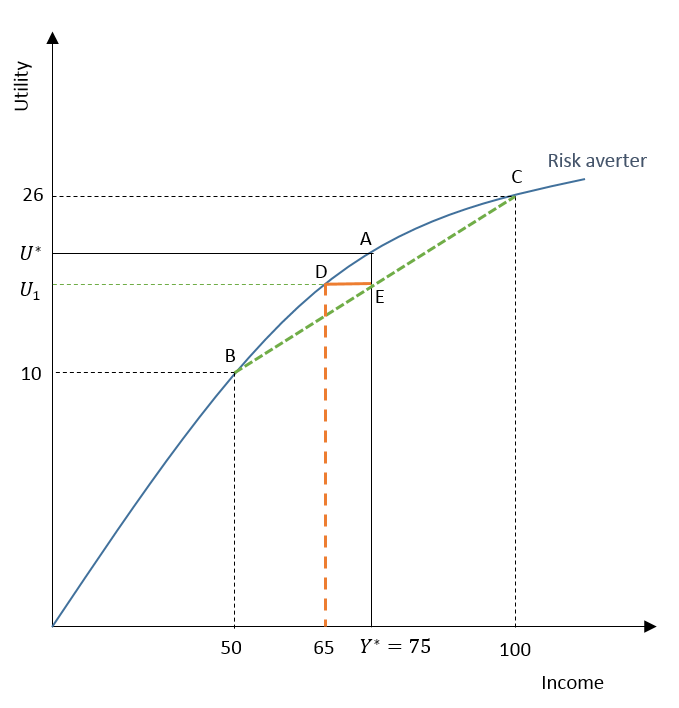
The Risk premium is shown by the distance of DE which is $10. Since the risk premium is $10, the individual will be indifferent between the new job and the current job only if the income from the current job was $65. This is equal to the earlier income minus the risk premium ($75 – $10 = $65). At this current income of $65 and expected income of $75 from the new job, the utility from both these jobs is equal at 18. Hence, the individual will be indifferent because the utility is the same for both jobs.
Econometrics Tutorials with Certificates

This website contains affiliate links. When you make a purchase through these links, we may earn a commission at no additional cost to you.