Blog

The Cobb Douglas production function is named after American economists Charles Cobb and Paul Douglas. They introduced this production function in 1928 in a paper published in the American Economic Review. The paper was titled “A Theory of Production” and was based on their empirical research into the relationship between inputs (labour and capital) and output in the manufacturing sector.

The Cobb Douglas function is one of the most widely used production functions to study production behaviour. It is definitely one of the most famous because it has several desirable properties and is easy to implement in practice. The Cobb Douglas production function can be expressed as follows:

This website contains affiliate links. When you make a purchase through these links, we may earn a commission at no additional cost to you.

Characteristics and properties of the cobb douglas production function

Homogeneous Production Function

Firstly, the Cobb Douglas production function is a homogeneous production function. This implies that if the scale of inputs is increased by a certain factor, the output will also increase by the same factor. The degree of homogeneity depends on the returns to scale. It is a homogeneous function of degree 1 if there are constant returns to scale.

Here, it is evident that the output will increase by the factor of “t” in the case of constant returns to scale because 𝜶+𝜷=𝟏. This shows that the function is homogeneous of degree one in the presence of constant returns. In the case of increasing or decreasing returns, this degree will depend on the value of 𝜶+𝜷.

Output Elasticities

Secondly, the output elasticities with respect to labour and capital are shown by their powers in the Cobb Douglas production function. Hence, the value of 𝜶 shows the output elasticity with respect to labour. This can be easily proven using the formula for calculating the elasticity:

Similarly, we can easily derive the proof for output elasticity with respect to capital:

In other words, these parameters 𝜶 and 𝜷 show the responsiveness of output due to a change in labour or capital. With a one percent increase in labour, keeping capital constant, the output will increase by 𝜶. Similarly, a one percent increase in capital, keeping labour constant, will increase the output by 𝜷.

Marginal Products and the Law of Diminishing Returns

Thirdly, the Cobb Douglas production function follows the Law of Diminishing Returns to a Factor. As more of an input is employed in production, keeping the other input constant, the marginal product of the successive units of that input will go on decreasing. For example, the marginal product of labour will go on decreasing as more labour is used, given that capital stays the same.

Furthermore, this can be easily proved using the second order derivatives with respect to labour and capital:

In the case of Labour, we can derive the second-order derivative as shown above. We know that “alpha” will always be less than 1 in case of constant and decreasing returns to scale because “alpha + beta” is equal to 1 in constant returns and less than 1 in decreasing returns. Even in increasing returns, this “alpha” is rarely greater than 1. As a result, the whole term will end up being negative since “(a-1)” will be negative. Since this second-order derivative is negative, we have diminishing returns with respect to labour. Similarly, we can derive this for capital and show diminishing returns with respect to capital.

Marginal Product can be expressed in terms of Average Products

Fourthly, the Marginal Products of inputs are related to their Average Product in the Cobb Douglas production function. The marginal product can be easily expressed in terms of the average product of the input as follows:

Therefore, we can observe that the marginal and average products are related by their respective output elasticities 𝜶 and 𝜷.

Average Product can be expressed in terms of the Capital-output ratio

Finally, if there are constant returns to scale, the average products of labour and capital can be expressed in terms of the Capital-labour ratio as follows:

It is important to note here that this is applicable only in case of constant returns to scale.

Marginal Rate of technical substitution (MRTS) and Elasticity of substitution

MRTS or Marginal Rate of Technical Substitution shows the amount by which one input must be reduced to increase the other input by one unit, to produce the same output. In other words, it shows the trade-off between the inputs. For example, MRTS will show the amount of capital that must be reduced to increase the labour by one unit and still produce the same output. Further, the MRTS for the Cobb Douglas production function can be derived as follows:

Therefore, the MRTS can be expressed in terms of the Capital-labour ratio and the output elasticities with respect to inputs.

Additionally, we can also easily derive the elasticity of substitution for the Cobb-Douglas production function. The elasticity of substitution can be defined as the ratio of percent change in the capital-labour ratio to the percent change in MRTS.

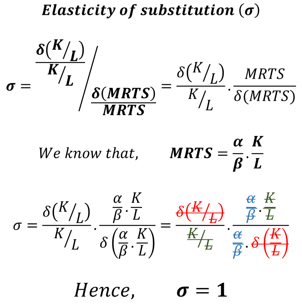
As we can see above, the Cobb Douglas production function has unit elasticity of substitution which is one of the shortcomings of the function. In reality, the elasticity of substitution between the inputs usually varies with changes in the input levels.

estimating the cobb douglas production function

One of the further advantages of the Cobb Douglas production function is that it is easy to estimate in practice. We can estimate it using the method of Ordinary Least Squares after taking the logarithm of the function. The parameters (A, 𝜶 and 𝜷) of the function can be estimated as follows:

This equation can be easily estimated using OLS or Ordinary Least Squares. Here, the estimated coefficients of the model represent the parameters of the Cobb Douglas production function.

Moreover, we can also assess whether the data shows constant, increasing or decreasing returns to scale. This is easy to figure out using the estimated coefficients of 𝜶 and 𝜷.

• If 𝜶 + 𝜷 = 1, Constant returns to scale
• If 𝜶 + 𝜷 > 1, Increasing returns to scale
• Finally, if 𝜶 + 𝜷 < 1, Decreasing returns to scale

Limitations of cobb douglas production function

Although the Cobb Douglas production function is widely used, it has a lot of shortcomings:

Elasticity of substitution is one: this is one of the major drawbacks of this function. Firstly, its unit elasticity of substitution makes this function very restrictive. In reality, the elasticity of substitution is not one, but it changes with a change in the level of inputs. As a result, the Cobb Douglas production function is not flexible in this respect at all.

Constant technology: secondly, the production function assumes the technology parameter (A) to be given and constant. This means that we cannot study the changes in technology and its effects using the Cobb Douglas production function. Industries that witness rapid technological changes cannot be suitably analysed using this function.

Static nature: thirdly, as with static technology, Cobb Douglas function does not take into account the dynamic market conditions and their effects on output. It cannot be used to understand how firms make adjustments to their output in reaction to changing input prices or other market conditions.

Aggregation bias: the function assumes that all the inputs of the same type are identical and interchangeable which is unrealistic. For instance, any two units of labour are not the same or identical.

Finally, even after considering the various shortcomings, the Cobb Douglas production function is a useful and essential tool. Moreover, it has motivated the development of several production functions. Other functions such as the CES, VES and the Translog production function have attempted to remove some of these shortcomings.

This website contains affiliate links. When you make a purchase through these links, we may earn a commission at no additional cost to you.