The ACF or Autocorrelation Function is one of the most widely used methods to check for stationarity of a time series. Moreover, it also gives valuable insights into the autoregressive (AR) and moving average (MA) structure of a time series. Along with the Partial Autocorrelation Function (PACF), it helps decide the AR and MA terms in ARIMA and SARIMA models.
In time series analysis and forecasting, it is essential to recognize a non-stationary time series and make it stationary. This is because a non-stationary time series does not give reliable results. We often use unit root based tests of stationarity such as ADF, KPSS tests etc. Aside from these, the Autocorrelation Function (ACF) is also an essential tool to check for stationarity.

Econometrics Tutorials with Certificates

Estimating the autocorrelation function (ACF)
The Autocorrelation Function (ACF) can be estimated at any lag using the following formula:

Moreover, the value of ACF or ρk lies between +1 and -1 (-1 < ρk < +1). In practice, we apply these tests on a sample, therefore, we sometimes refer to it as Sample Autocorrelation Function (SACF).
Choice of Lag
Usually, ACF is estimated up to one-third or one-fourth of the sample size. Suppose, a time series has 60 observations or time periods, then, k or lag of around 15 to 20 can be used. Sometimes, AIC or SIC (Akaike or Schwarz Information Criteria) are also used to choose the appropriate lag length.
Correlogram: Plotting the autocorrelation function
The ACF and PACF plots are also sometimes referred to as Correlograms. By plotting the correlogram, we can get insights into whether the time series is stationary or not. For a stationary time series, the values of ACF or ρk are close to zero and further hover around 0 at different lags. In the case of a non-stationary time series, the values of ACF tend to be high and, therefore, move closer to +1 or -1.
Plotting the confidence intervals along with ACF also helps in identifying stationarity. If the ACF lies beyond the confidence intervals at any lag, then we can conclude that the time series is non-stationary. On the other hand, a time series is stationary if the ACF values at all lags lie within the confidence intervals.
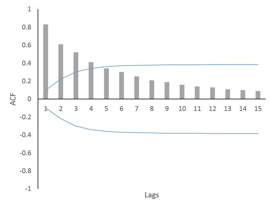
The above figure shows the Autocorrelation Function and its values for 15 lags. Additionally, the blue lines depict the confidence intervals. Furthermore, it is evident from this plot that the time series is non-stationary. We can conclude this because the first four lags of the ACF are significant.
Implementation in ARIMA and SARIMA models
The ACF and PACF plots are also helpful in determining the autoregressive (AR) and moving average (MA) structure of a time series. As a result, these plots are often used in ARIMA and SARIMA models to decide their structure. These plots provide a good starting point for deciding the number of AR (autoregressive) and MA (moving average) lags.
Econometrics Tutorials with Certificates

This website contains affiliate links. When you make a purchase through these links, we may earn a commission at no additional cost to you.