In the short run, capital is a fixed factor of production and only labour can be varied by firms to change output. The Law of Variable Proportions holds in the short run. The marginal product of labour starts declining after a certain number of workers have been employed with fixed capital. In the long run, however, all factors of production are variable. The firms can choose to expand their existing capital to produce more. Moreover, they can also substitute labour and capital to choose any combination of the two factors of production to produce the desired output. Isoquants and returns to scale help us understand production in the long run.
Because both labour and capital are variable in the long run, firms have to make the choice between labour and capital. That is, firms have to choose the quantity of both labour and capital that they will use to produce the given output.
This choice is similar to consumer choice. Consumers choose a combination of two products to maximize their utility, given the budget constraint. Consumers’ choice is determined through their indifference curves and a budget line. In the case of producers, they have to choose a combination of two inputs to maximize their output, given the budget constraint (depending on the cost of inputs). Hence, producer choice is determined using isoquants and isocost lines.
Here, we will discuss the isoquants facing a firm and returns to scale. Isocost line, isoquants and resulting producer equilibrium are discussed separately.
Econometrics Tutorials with Certificates

Isoquants
What is Isoquant?
An isoquant shows the different combinations of inputs (labour and capital) that produce the same output. This implies that given output can be produced using various possible combinations. Firms can use more labour and less capital or less labour and more capital to produce the same output.
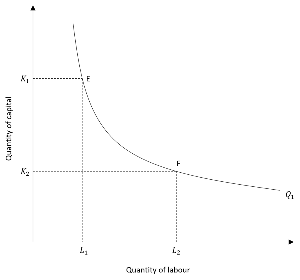
In the first diagram, the isoquant (Q1) shows the different combinations of labour and capital that produce the same output of Q1. At E, the producer uses more capital (K1) and less labour (L1) to produce the given out. However, the same output Q1 can also be produced using less capital (K2) and more labour (L2) shown by point F. Therefore, labour and capital can be used in various combinations to produce the same level of output.
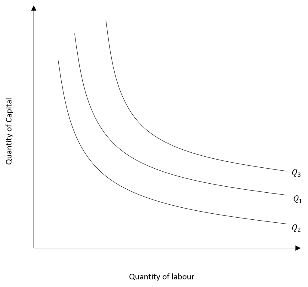
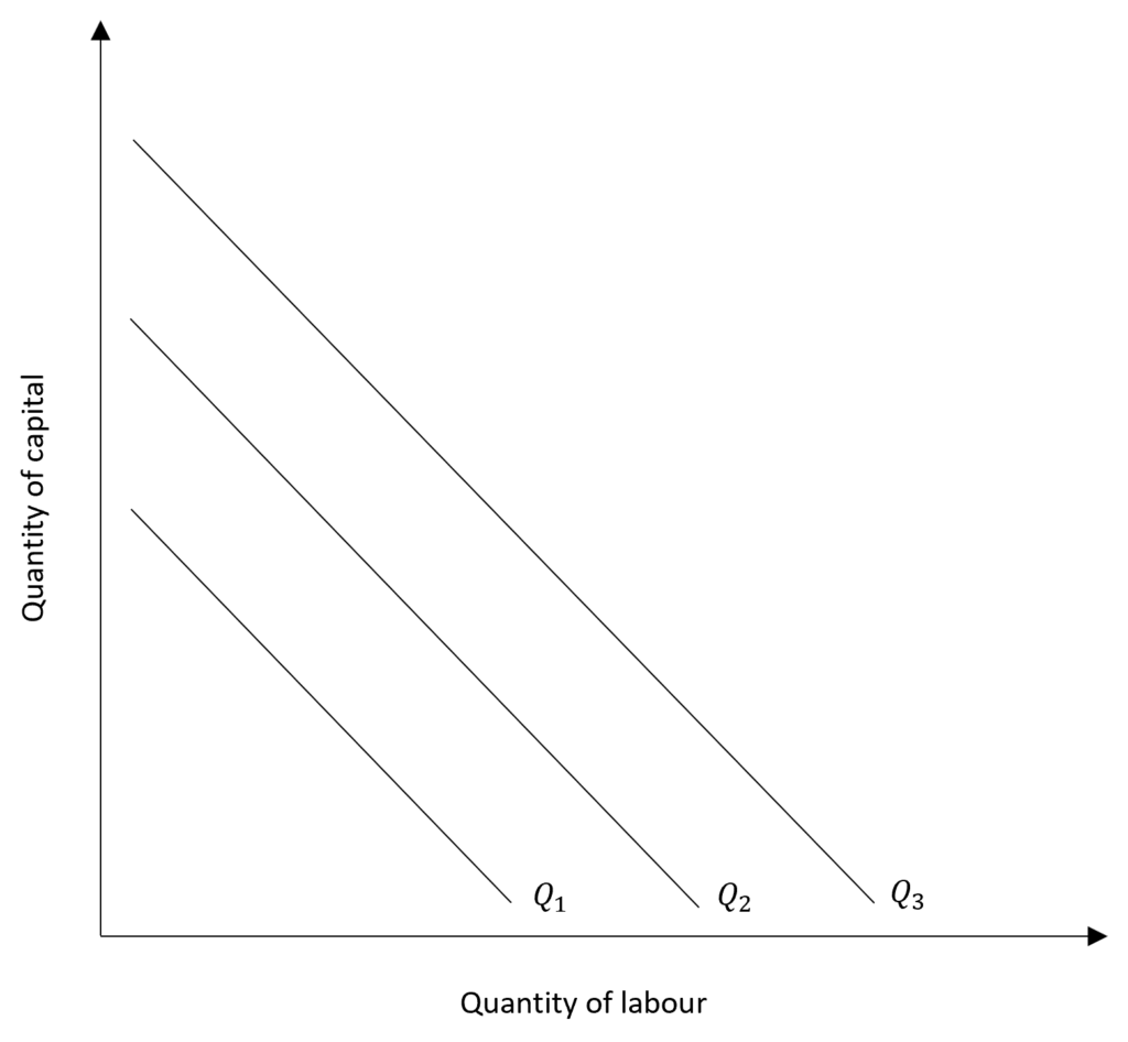
Isoquant map: isoquant map shows different levels of output, i.e. it consists of many isoquants. It is similar to indifference maps, which show various levels of utility. Higher isoquant means higher output and lower isoquant means less output. In the diagram, isoquant Q2 shows a lower output as compared to Q1. Whereas, Q3 shows a higher output level and the corresponding combinations of labour and capital that can be used to produce it.
Properties of Isoquants
The properties of isoquants are a lot similar to those of the Indifference curve and can be stated as:
- Isoquants are downward sloping from left to right. This means that with an increase in one input, the other input falls while the output remains constant. There is a trade-off between the inputs to maintain a given level of output.
- The isoquants are convex to origin because of the diminishing MRTS or Marginal Rate of Technical Substitution. We will discuss the MRTS and its diminishing nature below.
- Similar to indifference curves, isoquants do not intersect each other. Moreover, they also do not intersect the x-axis or the y-axis.
- Higher isquants represent higher level of output. We can also observe this in the isoquant map above where the higher isoquants (towards the right) show higher output.
Marginal rate of technical substitution (MRTS)
Labour and capital can be substituted with each other to produce the same output. Producers can employ more labour by reducing capital. Or, they can use more capital by reducing labour to maintain the same level of output. This shows that there is a trade-off between the use of labour and capital to produce the same level of output. This trade-off is known as the Marginal Rate of Technical Substitution (MRTS). MRTS is the slope of an isoquant.
The idea of MRTS is similar to the Marginal Rate of Substitution (MRS) in consumer theory. MRS shows the trade-off between two goods at a given level of utility. Here, MRTS shows the trade-off between two factors to produce the same output. Similarly, we ignore the negative sign on MRTS because isoquants are downward sloping and MRTS is always negative. We are concerned with the magnitude of the slope which determines the trade-off between the inputs.
MRTS can be defined as the quantity by which an input can be reduced when the other input is increased by one unit. For instance, MRTS of labour for capital is the quantity by which capital can be reduced when labour is increased by one unit, to produce the same output. MRTS can be estimated as follows:

MRTS is negative because one of the inputs will fall. We will have a negative change in capital in this case because we are considering MRTS of labour for capital. We include the negative sign in the formula to offset this negative value of MRTS. This is because we are only concerned with the magnitude of slope or trade-off.
diminishing MRTS
Similar to indifference curves, isoquants are downward sloping and convex to the origin. This results in a diminishing MRTS which happens because of diminishing marginal returns. The marginal product of an input falls as more of that input is used. When one input is reduced, more and more of the other input is needed to maintain the same output. This happens because the productivity of any input has its limits.
At a lower quantity of labour, the marginal product of labour is high. This means that when capital is reduced by one unit, less quantity of extra labour is required to offset that fall in capital and keep the output constant. On the other hand, the marginal product of labour is low when a large quantity of labour is being used. Due to low marginal product, more labour is needed to offset that one unit fall in capital and maintain constant output. Hence, diminishing marginal returns (also discussed in the law of variable proportions) cause the isoquants to be downward sloping and MRTS to be diminishing.
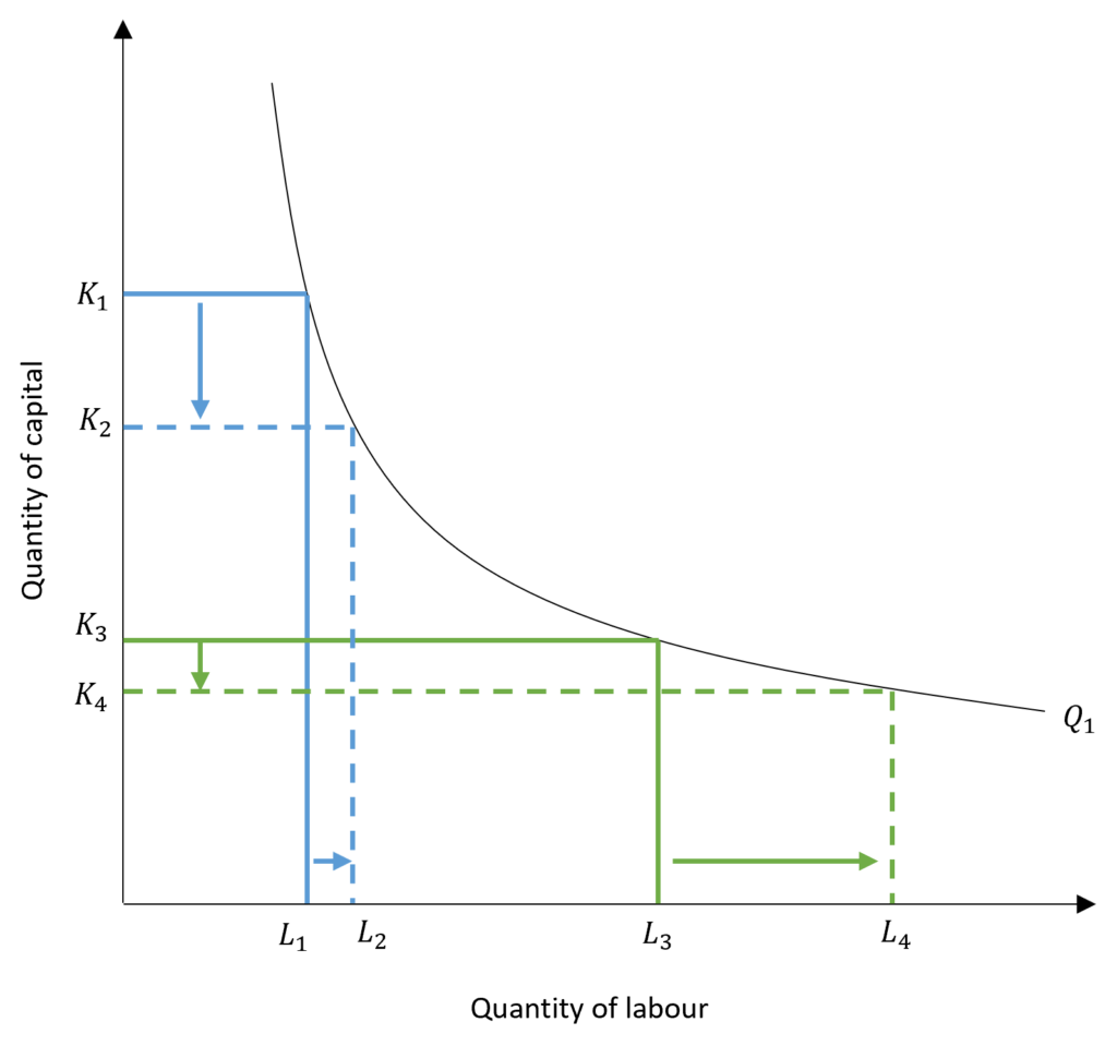
The diagram above shows the changing trade-off as a result of diminishing marginal returns. Initially, the labour employed is low at L1. A massive drop in capital from K1 to K2 can be offset by a small increase in labour from L1 to L2 because the marginal product of additional labour is high. As more and more labour is employed, the marginal product of labour goes on decreasing. As a result, a small drop in capital from K3 to K4 requires a huge quantity of additional labour (L3 to L4) to offset it and maintain the same output of Q1.
MRTS and Marginal product
MRTS and marginal products of labour and capital are closely related. Suppose, a producer reduces the capital and increases the use of labour in such a way that output remains constant. Then, additional output due to an increase in labour can be estimated as:
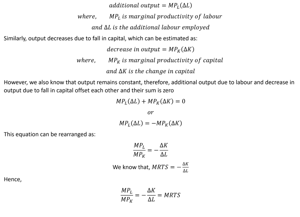
This means that MRTS is equal to the ratio of marginal products of labour and capital (factors of production). When labour increases and is used as a substitute for capital, MPL will go on falling. This is due to diminishing marginal returns. MPK will stay high because less capital is being used. Then, the ratio of marginal products will be low and the slope of isoquant (MRTS) will be low. Conversely, this ratio will be high when less labour is used along with more capital because MPL will stay high and MPK will be low. Hence, the isoquants are convex downward sloping curves because the slope (or MRTS) decreases as a firm moves along the isoquant.
Note: this relationship is essential in determining the producer equilibrium which will be discussed separately.
Special cases
Perfect Substitutability of Factors
In case of some goods, factors of production are perfect substitutes. This means that output can be produced by employing mostly labour or mostly capital or a balanced combination of these two. In such cases, the MRTS is constant and the isoquants are downward sloping straight lines.
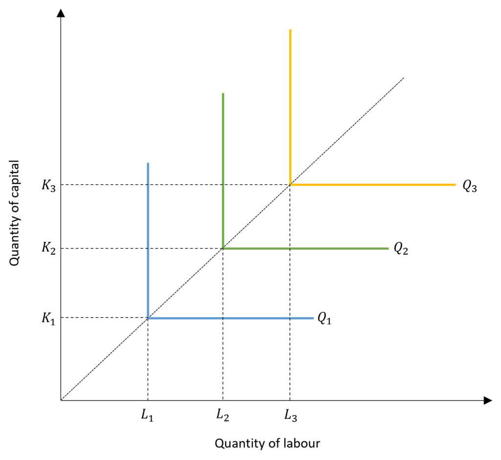
Leontief Production Function
This is also known as the fixed-proportions production function. As the name suggests, the proportion of inputs remains fixed. Output can be produced using a fixed combination of labour and capital and there is no substitutability between the two. To increase the output, both labour and capital have to be increased in the same proportion. Consider the example of a food recipe which requires a fixed amount of ingredients as inputs for each pack. More can be produced only if all the ingredients are available in the required proportions fixed by the recipe.
Return to scale
Returns to scale can be defined as the rate at which the output of a producer will rise if the factors of production or inputs are increased proportionately. In the long run, all inputs are variable. The producer can decide to expand the output by increasing the scale of production. For instance, consider a producer employing 1 worker on 1 machine to produce output. He or she can expand the scale of production by employing 2 workers on 2 machines. In this example, the output will most definitely increase. By doubling the inputs, however, the output will not necessarily double. The increase in output can be exactly double, less than double or even more than double.
These three scenarios can be explained as increasing, decreasing or constant returns to scale.
Increasing Returns to Scale
Increasing returns to scale is a situation where the rate at which the output increases is more than the rate of increase in inputs. If the inputs are doubled, the output will increase by more than double in the existence of increasing returns.
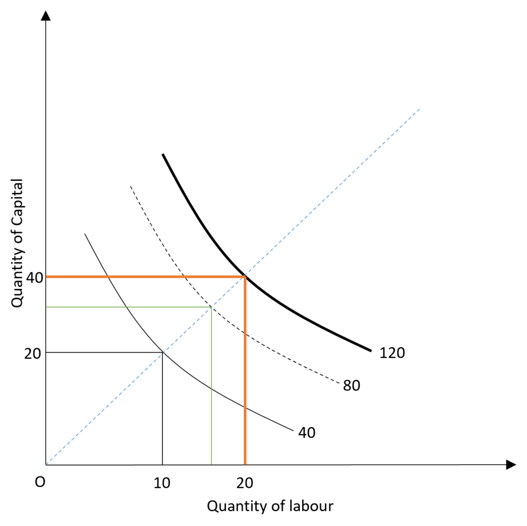
The isoquants are closer to each other in case of increasing returns. This is because the output is doubled with less than double inputs employed. In the diagram, the output is doubled from 40 to 80 units when the labour and capital are less than doubled. When the inputs are doubled from 10 to 20 (labour) and 20 to 40 (capital), the increase in output is more than double from 40 to 120 units.
Constant Returns to Scale
If the rate at which output expands is equal to the rate of increase in inputs, then a producer is realising constant returns to scale. If inputs are doubled, the output will also double in case of constant returns.
The isoquants are equally spaced in constant returns because a 100 per cent increase in inputs leads to an equal increase in output by 100 per cent.
Decreasing Returns to Scale
the rate of increase in output is less than the rate of increase in inputs in case of decreasing returns to scale. With double inputs employed, the output produced will be less than double when decreasing returns operate.
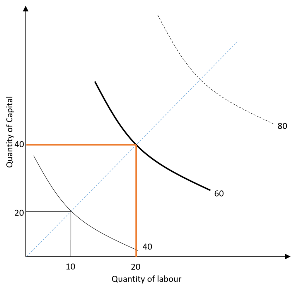
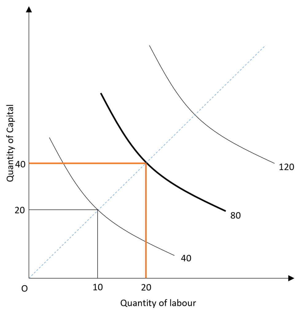
The distance between the isoquants is greater in the case of decreasing returns because the increase in output is less than the increase in inputs. That is, inputs have to be increased by more than 100 per cent to increase output by 100 per cent. In the diagram, the output is doubled when inputs are more than doubled. When inputs are doubled from 10 and 20 (labour) to 20 and 40 (capital), the output is less than doubled from 40 to 60 units.
Note: a firm can experience all three types of returns to scale at different stages of expansion. For example, a firm may have increasing returns when it expands its production initially. However, as it goes on expanding and becomes large, increasing returns can be replaced by constant returns to scale. Eventually, decreasing returns might start to operate due to several reasons such as coordination or communication difficulties as a firm keeps growing.
Econometrics Tutorials with Certificates

This website contains affiliate links. When you make a purchase through these links, we may earn a commission at no additional cost to you.