Autocorrelation Function (ACF) and Partial Autocorrelation Function (PACF) can provide valuable insights into the behaviour of time series data. They are often used to decide the number of Autoregressive (AR) and Moving Average (MA) lags for the ARIMA models. Moreover, they can also help detect any seasonality within the data. Correct application and interpretation are essential in extracting useful information from the ACF and PACF plots.
The ACF and PACF plots can be obtained from the original data, as well as from the residuals of a model. On the original data, these plots can help detect any autoregressive or moving average terms that may be significant in the time series. When applied to the residuals, these plots can detect any remaining autocorrelation in the model. This also provides insight into whether additional AR or MA terms need to be included in the model. Similarly, they can detect any seasonal behaviour that must be accounted for in the model.

Definition of autocorrelation function (ACF) and Partial autocorrelation function (PACF)
The ACF shows the correlation between the time series and its own lagged values. It represents a correlation coefficient between the series and its past values. For instance, ACF at lag 3 is calculated as the correlation between the series (Yt) and the same series lagged by 3 time periods (Yt-3). In this way, the correlation is estimated at every lag and plotted on a graph showing the correlation coefficient at each lag. Pearson or Spearman Rank Correlation can be used to estimate the correlation between the two series (original and lagged).
The PACF is estimated by controlling the effects of other lags, generally using linear regression. The PACF at a given lag is the coefficient of that lag obtained from the linear regression. The regression includes all the lags between the current time period and the given lag as independent variables. For instance, PACF at lag 3 can be estimated as:
Yt = B0 + B1Yt-1 + B2Yt-2 + B3Yt-3
Here, B3 = PACF at lag 3
PACF at all lags can be estimated with separate regressions including all the lags up to the coefficient of the lag that we need. For example, to estimate PACF at lag 8, we will include 8 lagged variables and the coefficient of the 8th lag will give us PACF at lag 8.
The PACF graph is constructed by plotting all the values of PACF obtained from regressions at different lags.
identifying AR, MA and ARMA Terms with ACF and PACF plots
AR process
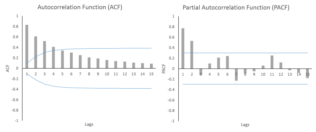
A gradual geometrically declining ACF and a PACF that is significant for only a few lags indicate an AR process. In the figures, we can see that ACF is geometrically declining with lags. The PACF has 2 significant lags followed by a drop in PACF values and they become insignificant. With 2 significant PACF lags and gradually falling ACF, we can say that the series is an AR(2) process. The lags of AR are determined by the number of significant lags of PACF.
MA process
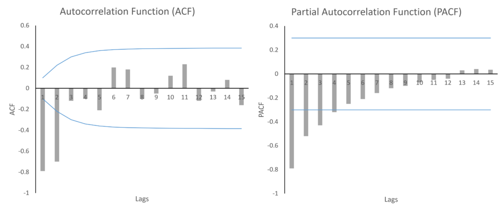
MA process shows a gradually geometrically declining PACF and the ACF has a few significant lags. This is the opposite of the AR process above. Here, the PACF is falling geometrically and the ACF has 2 significant lags before dropping. This indicates MA(2) process. For instance, if the ACF had 1 significant lag, it would mean MA(1) process because MA lags are determined by the number of significant ACF lags.
ARMA process
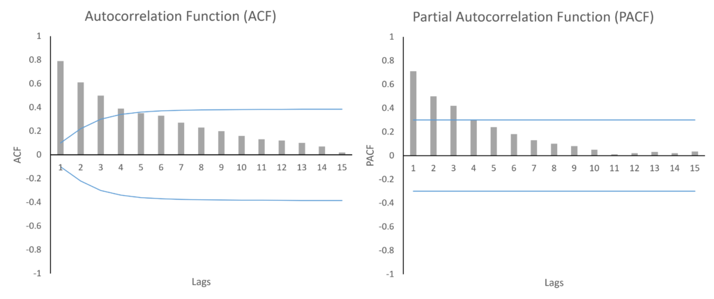
An ARMA process is indicated by geometrically filling ACF and PACF. In this figure, both ACF and PACF are gradually falling with lags. The number of AR and MA terms to include in the model can be decided with the help of Information Criteria such as AIC or SIC.
Important: the ACF and PACF plots give a good starting point to determine the AR and MA process and terms. However, the number of terms to include in the final model should be determined after considering other factors. For instance, more AR/MA terms have to be included if the model suffers from autocorrelation. In some cases, models with different AR and MA lags can give better forecasts and we might end up with an AR, MA or ARMA model of a different order than indicated by these plots.
Identifying seasonality with ACF and PACF plots
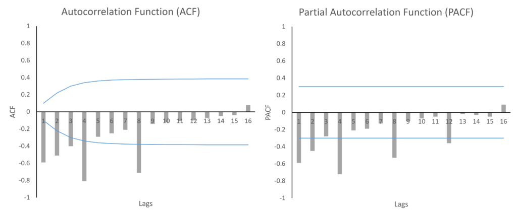
Seasonal AR process
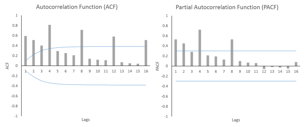
In the above figures, we can see highly significant lags every 4 time periods. This indicates a 4 time period seasonal cycle in the data. The ACF is gradually declining with every 4th period and the PACF shows 2 significant seasonal lags (4th and 8th lag). This suggests that the series is a Seasonal-AR(2) process because the PACF has 2 significant lags.
Additionally, this series is also an ARMA process because the other lags of both ACF and PACF are geometrically declining.
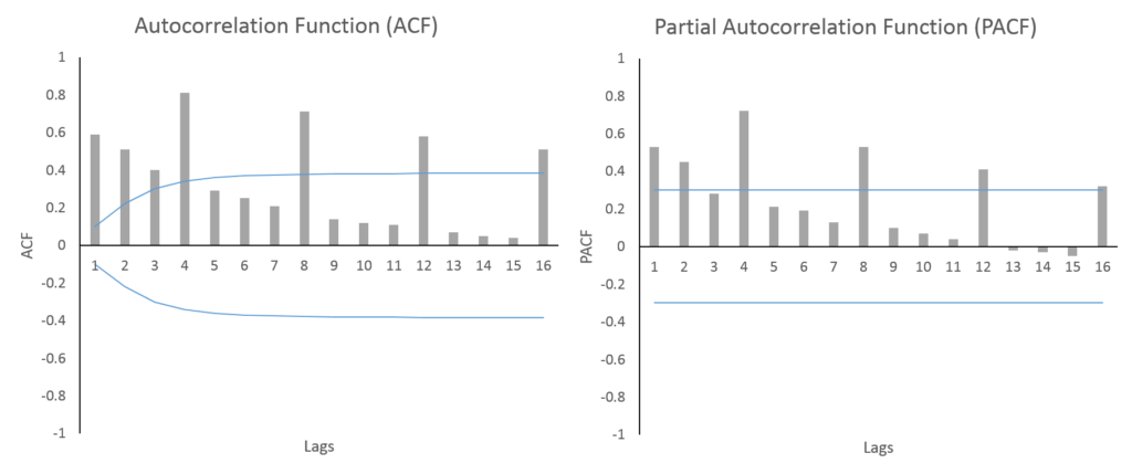
Seasonal MA process
These figures also indicate a 4 time period seasonal cycle. But, this series is a Seasonal-MA(2) process because we can observe 2 significant seasonal lags in ACF (4th and 8th lag) and the PACF is gradually falling every 4th period. In addition to the ARMA process, we will also need to account for 2 significant Seasonal-MA lags in the model.
Seasonal ARMA process
A Seasonal-ARMA process has both ACF and PACF declining gradually over seasonal lags. The above figures show a Seasonal-ARMA process with a 4-period cycle. The ACF and PACF are significant and declining gradually with every 4th lag. Usually, Seasonal-AR(1) and Seasonal-MA(1) lags are enough to account for such behaviour.
Important: optimization and convergence can sometimes be difficult with too many AR, MA, ARMA and seasonal-AR/MA terms. This is especially true for seasonal-AR and MA terms in a SARIMA model. Hence, we must be careful not to include too many lags because one lag of SMA or SAR is usually enough. To choose the appropriate lags and models, we can rely on Information criteria or the Forecasting Accuracy of the different ARIMA or SARIMA models.
Econometrics Tutorials with Certificates


This website contains affiliate links. When you make a purchase through these links, we may earn a commission at no additional cost to you.