The Phillips curve is a graphical representation of the inverse relationship between inflation and unemployment. The curve is named after economist A.W. Phillips, who first observed this relationship in the United Kingdom in the 1950s. The Phillips curve advocates that there is a trade-off between inflation and unemployment. It implies that when unemployment is low, inflation tends to be high. On the other hand, when unemployment is high, inflation tends to be low.
The Phillips curve has been the subject of much debate among economists. This inverse relationship postulated by the Phillips curve has caused a lot of debate related to its effectiveness and adoption in macroeconomic policies. Some have questioned whether the relationship between inflation and unemployment still holds true in today’s globalized and rapidly changing economy.
Econometrics Tutorials with Certificates

A Brief History of the Phillips Curve
A.W. Phillips was a New Zealand-born economist who first observed the relationship between unemployment and inflation in the United Kingdom in 1958. The paper was titled, “The Relation between Unemployment and the Rate of Change of Money Wage Rates in the United Kingdom, 1861-1957“. Phillips was studying the relationship between unemployment and wage changes. He found that there was a clear negative correlation between the two variables. In other words, when unemployment was low, wage growth tended to be high. When unemployment was high, wage growth tended to be low.
Other economists soon began to explore this relationship. In the 1960s, the Phillips curve became a popular tool for macroeconomic analysis. It was widely believed that policymakers could use the Phillips curve to make trade-offs between inflation and unemployment. For example, if inflation was too high, policymakers could reduce it by increasing unemployment. Conversely, if unemployment was too high, policymakers could reduce it by allowing inflation to rise.
However, in the 1970s, the Phillips curve became the subject of much criticism. In particular, economists began to question the stability of the trade-off between inflation and unemployment. They pointed out that the relationship between the two variables was not as consistent as previously thought and that other factors, such as supply shocks, could disrupt the relationship.
the short run Phillips curve
The Phillips curve, as given by A.W. Phillips, focused on the relationship between the rate of unemployment and the rate of increase in wages. He used this relationship to explain the increases in the price level or inflation rate.
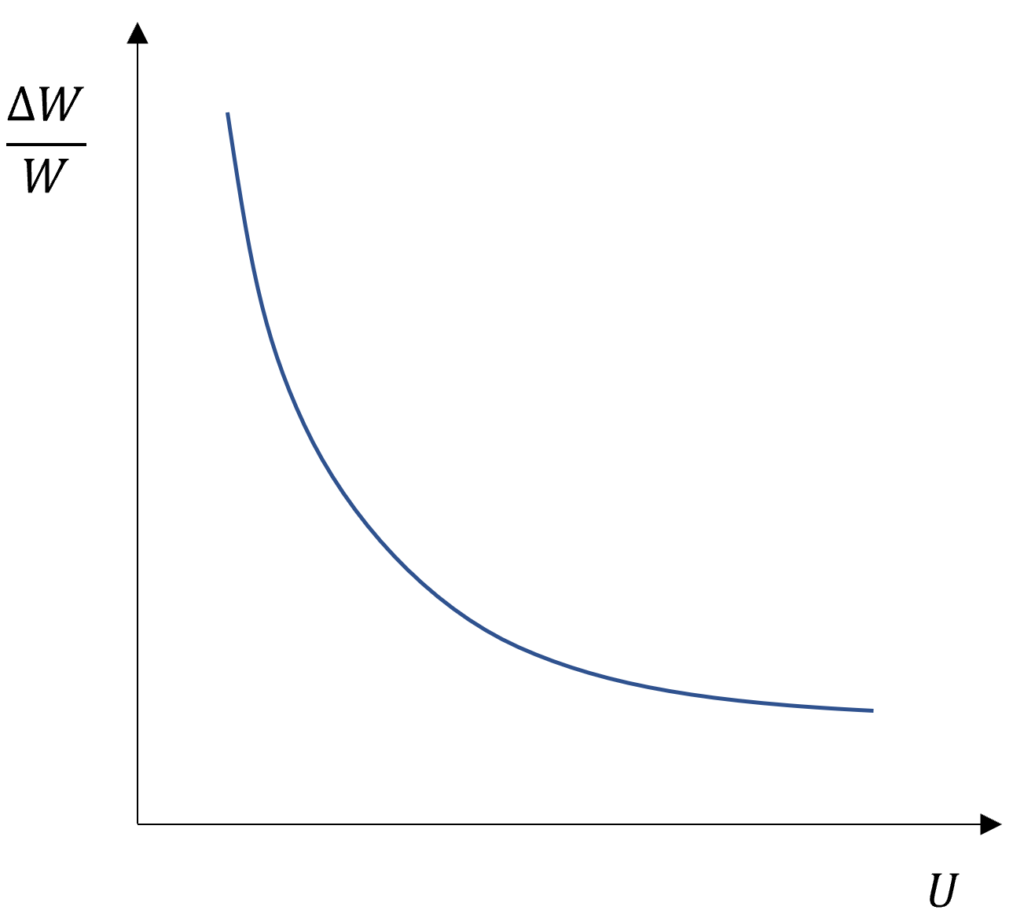
The Phillips curve, as shown in the diagram, depicts an inverse relationship between wage rate increase and unemployment rate. There is a trade-off between the wage level increase and the rate of unemployment. This implies that higher unemployment rates are coupled with lower increases in wage rates. On the other hand, a low unemployment rate is accompanied by higher increases in wage rates.
This inverse relationship is also transferred to the inflation rate because of the rate of increase in wages. There is a direct relationship between the rate of wage increase and the inflation rate. In the diagram, we saw that there is an inverse relationship between the rate of increase in wages and the rate of unemployment. This results in an inverse relationship between the inflation rate and the unemployment rate as well. Hence, we observe a trade-off between the inflation rate and the unemployment rate. There are two main reasons that result in this relationship which are discussed below.
Reasons for the Inverse relationship between Inflation and Unemployment rate
Demand for Labour
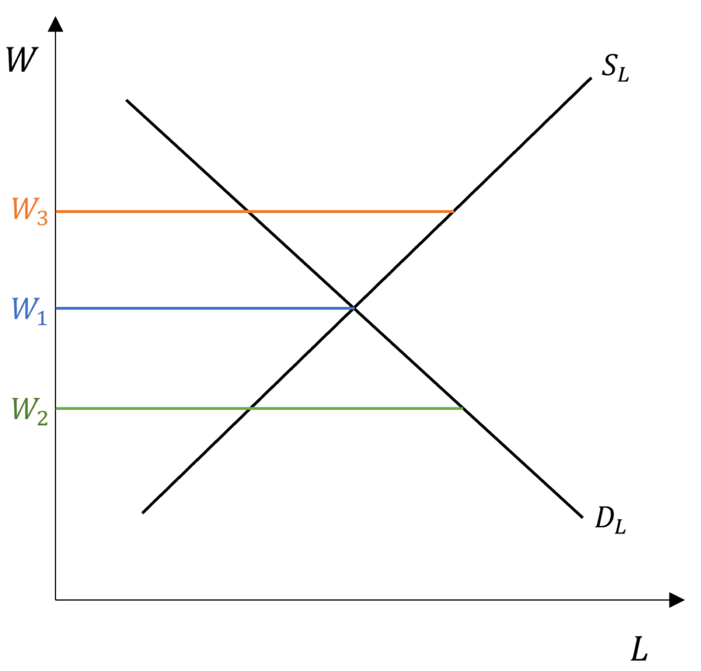
In the above diagram, W1 is the wage rate that shows equilibrium in the labour market. The demand and supply of labour are equal at this point. It is important to note here that this point does not imply the absence of unemployment. It simply means that the number of unemployed people is equal to the number of vacancies. Similarly, the wage rate W2 shows a situation of excess demand for labour because the demand will be much higher as compared to the supply of labour. Conversely, a higher wage rate of W3 means an excess supply of labour.
In the situation of excess demand, we will have a low unemployment rate because the demand for labour is greater than its supply. Because demand is high, it will push the wage rate upwards leading to an increase in the wage rate. This happens because the employers are willing to pay more for the workers. As a result, we see a leftward movement on the Phillips curve with an increase in the wage rate when unemployment is low.
On the other hand, the increase in the wage rate will be negative during an excess supply of labour and high unemployment. At the W3 wage rate, demand for labour will be low and the labour will be willing to work at lower wages. This pushes the wages downwards and leads to a fall in the wage levels. In such cases, the Phillips curve might eventually become negative with a rightward movement along the Phillips curve if the unemployment rate increases and inflation becomes negative.
Demand for labour and the shape of the Phillips curve
The movement in the wage rate increase will be greater with higher levels of excess demand and vice versa. Suppose, the wage rate is even lower than W2 and the excess demand is higher. In that case, the rate of increase in the wage rate will be higher as well. As a result, the Phillips curve becomes steeper as unemployment goes on to decrease. The higher the excess demand, the higher will be the changes in the wage rate movement. This is the reason why the Phillips curve is steeper as we move closer to the y-axis.
This happens due to the time involved for the labour to secure a job. When the excess demand is higher, the average time it takes the labour to find a job that they want is low. This happens because higher excess demand provides more opportunities to the workers. They will be able to find the job that they want more easily. In turn, this will lead to a faster rise in wage rates. When excess demand is low, employers’ demand for workers is relatively lower as well.
This means fewer opportunities and a longer search period. As a result, the increase in wage rate is slower as compared to the situation of higher excess demand.
There is, therefore, an inverse relationship between the level of excess demand and the speed of wage increase. This gives rise to the shape of the Phillips curve that we see in the diagram above.
Bargaining power of Labour
Labour has some bargaining power related to wages as they are usually organised into trade unions etc. This organised labour can demand higher wages from their employers and push the wages up. However, their bargaining power depends on the level of unemployment rate.
In times of low unemployment rate, the labour has more bargaining power and they can demand higher wages. This is possible because there is excess demand for labour and they can negotiate better wages. This situation of low unemployment is usually accompanied by higher demand for goods in the economy and higher profits for employers. Therefore, employers are also more flexible as they are looking for more labour in times of excess demand.
This drives wages upwards in times of low unemployment. Moreover, the lower the unemployment, the higher will be the bargaining power of labour. Thus, the Phillips curve gets its inverse relationship and shape.
On the other end of the spectrum is the situation of high unemployment. The bargaining power of organised labour is low during high unemployment when there is low excess demand for labour. As a result, employers are resistant to agreeing to even smaller increases in wages. Thereby, higher unemployment implies relatively lower bargaining power, lower increase in wages and lower inflation rate.
Rate of Increase in Wages and Rate of Inflation
In the sections above, we have established the inverse relationship between the rate of increase in wages and the rate of unemployment. We also discussed the reasons behind this trade-off. However, we are yet to talk about the process of how the rate of increase in wages translates to a rate of inflation.
Earlier, we mentioned that there is a direct relationship between the rate of increase in wages and the rate of inflation. This means that wage increases directly affect price levels or inflation. Since the unemployment rate affects the increases in wage rates, it also ends up affecting the inflation rate. With higher unemployment, we observe lower increases in wage rates and lower inflation rates. On the other hand, lower unemployment leads to higher increases in wage rates and higher inflation rates.
We must note here that increases in wage rates may not fully translate to an increase in the price level or inflation. The eventual increase in the price level will depend on the changes in productivity. If an increase in wage rate is accompanied by a zero increase in productivity, it will lead to an equal increase in price levels or inflation rate. However, it has been observed that the increase in labour productivity is not zero. But, the increase in wage rates tends to be higher than the increase in labour productivity.
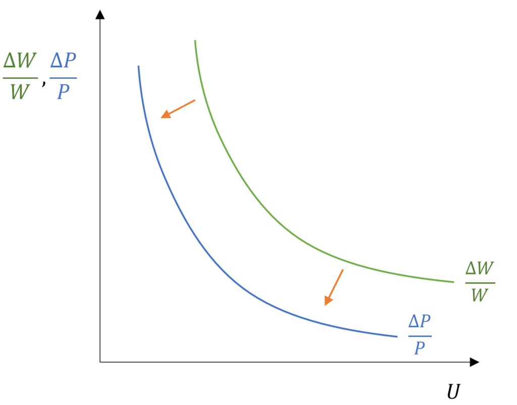
The diagram depicts a situation where there is an increase in productivity, but this increase is lower than the increase in the wage rate. Hence, the resultant inflation rate and price level (∆𝑃/𝑃) increase will be below the curve showing the increase in the wage rate. Finally, we can see the inverse relationship and trade-off between unemployment and inflation rate.
Long run Phillips Curve: Expectations Augmented Phillips Curve
The empirical evidence related to the Phillips curve has two sides. Some empirical studies support the existence of the inverse relationship as postulated by the Phillips curve. Whereas, other studies contradict it and claim that the relationship is not stable and there are other important factors involved. Overall, the various findings suggest that the Phillips curve relationship holds relatively well in the short run. But, this relationship tends to be unstable and breaks down in the long run.
Milton Friedman and Edmund Phelps introduced a long-run Phillips curve which is vertical and aligned with the empirical studies. He argued that the inverse relationship does not work in the long run. This long-run Phillips curve is often called the Expectations Augmented Phillips curve. This name is due to the fact that it incorporated people’s expectations into the relationship between unemployment and inflation rate. That is, Friedman included adaptive expectations (also used in his Permanent Income Hypothesis) into the Phillips curve relationship.
Deriving the Long run Phillips curve
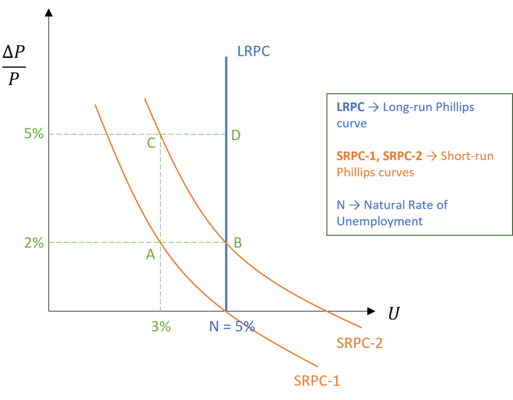
In the above diagram, the SRPCs represent the short-run Phillips curves which are similar to the original Phillips curve. The LRPC, however, is the long-run Phillips curve which is vertical or parallel to the y-axis. The level of N is known as the Natural Rate of Unemployment and the economies tend to settle at this unemployment rate in the long run.
We are assuming here that the natural rate of unemployment (N) is 5% and that is where the economy is operating initially. There is no increase in price level or inflation at this point. Suppose, the government tries to reduce unemployment below the current 5% level to 3% using various policies. From point N, the economy moves to point A because the government is able to reduce unemployment to 3% in the short run.
As a result, we see a movement to the left on SRPC-1 (short-run Phillips Curve). At A, the economy is operating at a 3% unemployment rate. But, this leads to higher inflation at 2%.
Role of Expectations
Hence, the government is able to reduce unemployment by accepting higher inflation in the short run. However, this is where the role of expectations becomes important. Initially, people do not expect any inflation at point N. The actual and expected inflation are equal at that point N. As the economy moves to point A and inflation rises to 2%, people revise their expectations.
As people realise that their real income has fallen due to the rise in inflation to 2%, they demand higher wages for themselves. This happens because they revise their expectation about inflation and expect higher inflation rates. With higher wages demanded by labour, the demand for labour falls and unemployment increases again. The economy ends up back at the 5% unemployment rate but with higher inflation of 2% shown by point B.
This will keep on going if the government tries to reduce unemployment and the economy will keep returning to the natural rate of unemployment (5%). The inflation will go on increasing from 2% to 5% (at points C and D) and so on, while the unemployment keeps coming back to 5% in the long run.
This gives rise to a vertical Phillips curve in the long run shown by LRPC in the diagram. Government policies can reduce unemployment below N (natural rate of unemployment) only in the short run. That is the reason why the short-run Phillips curves (SRPC-1 and SRPC-2) are downward-sloping. In the long run, the economy will keep coming back to the long-run Phillips curve because people revise their expectations about inflation.
Natural Rate of Unemployment
In the diagram above, we assumed that the Natural rate of Unemployment is 5% and is shown by N. In reality, this rate can be anything and can vary across different economies, change over time, and can be affected by several factors. This natural rate of unemployment is the point where the markets will be in equilibrium. If the policies attempt to decrease unemployment, it will lead to rising inflation in the short run as we observed above. On the other hand, if the unemployment is above this natural rate, then it would lead to deflation
The policies are only effective for a short period. In the long run, the unemployment rate will tend to return back to the natural rate. Thus, any policies aimed at reducing unemployment will be ineffective and will only lead to higher inflation. Moreover, inflation will be accelerating if the policies attempt to maintain unemployment below the natural rate. This means that inflation will increase at a faster rate. The reason behind this phenomenon is the shape of the short-run Phillips curve which gets steeper closer to the y-axis. The increase in inflation is greater as we move from Point A to C. This increase will be even higher if the policies keep trying to decrease unemployment.
However, this does not mean there is no way to reduce unemployment. To reduce unemployment, the policies should focus on reducing the natural rate itself. If we can reduce the natural rate of unemployment (from 5% to 3% for example), then we will be able to reduce unemployment without causing increased inflation. To achieve this, we must understand the factors that affect and determine the natural rate of unemployment.
Determinants of the Natural Rate of Unemployment
The Natural Rate of Unemployment is influenced by several structural factors. Some of the most important factors are:
Labour Market Institutions
The structure of labour markets, such as unionization rates, minimum wage laws, and employment protection laws, can affect the natural rate. In general, labour market institutions that create more rigidities or barriers to entry may increase, while those that promote flexibility and mobility may decrease the natural rate of unemployment.
Technological Change
Changes in technology can affect the natural rate of unemployment by altering the demand for labour and the skills required by employers. For example, if new technologies require highly skilled workers, the natural rate may be higher because it takes time for workers to acquire these skills.
Education and Training
The level of education and training of the workforce can affect the natural rate of unemployment by affecting the skills and qualifications of workers. In general, a more highly educated and skilled workforce may have a lower natural rate because they are better able to find employment.
Economic Policies
Macroeconomic policies, such as fiscal and monetary policy, can affect the natural rate of unemployment by influencing the overall level of economic activity. For example, reducing the barriers to entry to allow foreign firms into the market may lead to more employment opportunities and a fall in the natural rate of unemployment.
Demographics
The age, gender, and education levels of the labour force affect the natural rate of unemployment as well. For example, if there are more older workers in the labour force, the natural rate may be higher because older workers tend to have higher unemployment rates. Similarly, if there are more young workers who are still in school or training, the natural rate of unemployment may be lower because they are not actively seeking employment.
conclusion
The Phillips curve is an essential tool in understanding the relationship between inflation and unemployment. Since it was introduced, several economists have made contributions and modifications to it. Even to this day, it remains a highly discussed and debated concept in macroeconomics.
Moreover, the Phillips curve provides the essential knowledge that helps in adopting macroeconomic policies. While the policies directed towards reducing unemployment may be effective in the short run, they do not work in the long run. Instead, the macroeconomic policies should focus on the structural factors that affect the natural rate of unemployment itself. By lowering the natural rate of unemployment, it is possible to reduce unemployment without causing inflationary pressures.
These ideas about the Phillips curve and the Expectations Augmented Phillips curve were further developed by Tobin and Solow. They further argued that the long-run Phillips curve is not vertical, but it is still steep. The original Phillips curve did not consider expectations at all and put forward a downward-sloping Phillips curve. The long-run Phillips curve used Adaptive expectations and argued that people can fully adjust their expectations, leading to a vertical Phillips curve. However, Tobin and Solow argued that people do not have perfect expectations. As a result, the Phillips curve lies somewhere between the two formulations. That is, it is not vertical, but a steep download-sloping curve in the long run.
Econometrics Tutorials with Certificates

This website contains affiliate links. When you make a purchase through these links, we may earn a commission at no additional cost to you.