Production can be defined as the process by which inputs are used to make outputs. Inputs, also known as factors of production, include resources such as labour, capital and raw materials. Firms employ these factors of production in various combinations in the process of production of outputs. In the short run, not all factors can be changed. Some factors and overall production technology stay the same. The law of variable proportions helps analyze how the output changes when some inputs are changed in the short run, keeping other inputs constant.
Production function
A production function gives the relationship between inputs and the resultant output. A production function shows the maximum amount of output that can be produced using the given combination of inputs. Although production involves several factors, our analysis will focus on the two most important factors or inputs, i.e. labour and capital.
q = f(L, K)
Where ‘q’ is the output, ‘L’ is the labour employed and ‘K’ is the capital.
A firm can adopt various combinations of inputs to produce a given output. One firm might choose to employ more labour and less capital. Whereas another firm might choose to use capital-intensive methods that require less labour to produce the same quantity of output. Hence, different combinations of inputs can be employed in production.
It is important to note that technology is given as constant here. That is, a given production function applies only to a given level of technology. With changes or improvements in technology, a firm might be able to produce more output with the same quantity of inputs. Or, they might be able to produce the same output with fewer inputs. Research, development and adoption of new technology take a long time. Hence, technology is assumed to be constant in the short run.
Econometrics Tutorials with Certificates

Law of Variable proportions
In the short run, it is not possible to change all factors of production. For instance, capital such as plants and machinery cannot be varied in the short run. This is because setting up new production plants or purchasing new machinery can take months and years to implement.
However, a firm can employ more labour in the short run to increase its production. As a result, the output is a function of labour in the short run and the capital remains constant. Capital is a fixed factor and labour is a variable factor in the short run.
Therefore, the law of variable proportions shows how the output changes with changes in variable input of labour, while capital is fixed.
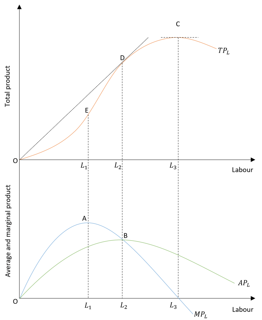
Total Product (TPL): the total product of labour curve shows the total output of the firm at different quantities/number of labour employed. The capital stays constant or fixed in the short run.
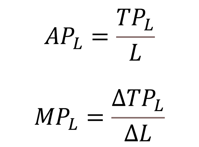
Average Product (APL): average product of labour curve shows the productivity of the workforce. That is the total output per labour. It is obtained by dividing the total product (TPL) by the quantity of labour employed (L).
Marginal Product (MPL): marginal product of labour curve shows the changes in the total product (TPL) as a result of changes in labour employed. It can also be defined as the change in the total product (TPL) with one unit increase in labour.
It can be estimated as the first order derivative of the total product (TPL) with respect to labour.
phases of the law of variable proportions
Initially, the total product is zero when labour employed is zero. With an increase in labour employed, total product or TPL increases at an increasing rate in the beginning till it reaches point E.
Point E is known as the point of inflection because the total product (TPL) increases at a decreasing rate after this point. Before E, the marginal product curve (MPL) is rising as the total product increases at an increasing rate. This implies that the increase in total product rises with each successive unit of labour. At E, L1 labour is employed and the marginal product curve (MPL) reaches its maximum and starts falling as more labour is used.
The average product curve (APL), which shows labour productivity, increases or rises initially. It reaches the maximum at point D when L2 labour is used. As seen from point B which corresponds to D, average product and marginal product are equal at L2 quantity of labour. Therefore, labour productivity is maximum when APL and MPL are equal. Beyond this point, the average product also starts falling as more labour is hired. However, the decrease in the marginal product (MPL) is greater than the decrease in the average product (APL).
As more and more labour is used, the marginal product goes on falling and reaches zero at L3 quantity of labour. As the marginal product becomes zero, it means that the additional labour does not lead to an increase in total product. Hence, the total product curve (TPL) is at its maximum and starts falling after this. Moreover, the marginal product or MPL becomes negative if more labour is employed.
relationship between average and marginal product
When MPL is greater than APL, the average product or APL is rising. This means that the output of the additional worker (shown by MPL) is greater than the average output (shown by APL). Therefore, the employment of that additional worker leads to an increase in productivity or an increase in the average product. This is why the average product (APL) rises when MPL is greater than APL.
On the other hand, when the marginal product becomes less than the average product, an additional worker will cause a fall in the average product because of his or her lower contribution to the total product. Therefore, the average product curve is downward sloping or falling when MPL is less than APL.
law of diminishing returns
The law of diminishing returns to a factor states that additions to the output eventually start falling as more input is used. This is shown by the marginal product curve which starts falling after point E. But why does this happen?
Given a fixed amount of capital, the marginal product increases in the beginning because the capital is underutilised. With more labour, the total product rises rapidly with efficient use of existing capital. For instance, if a machine needs 5 people to operate effectively, then, using 1 person will lead to its underutilisation. As more labour is employed, its utilisation will improve.
Similarly, the marginal product will eventually start falling and become negative. This happens because labour becomes less effective if too many are employed. Suppose, 10 people are hired to use that same machine which requires only 5 people. Then, the marginal product of that additional labour will be low and may even be zero or negative. This happens because too many workers will start interfering with the production process.
It is important to note that marginal product does not fall due to poor quality of labour in the later stages. It occurs because of the overutilization of fixed capital as capital cannot be utilised beyond its capabilities. For example, if a machine has a maximum production of 10 units of output per hour, this cannot be increased with additional labour because it is the production limit of that machine.
Econometrics Tutorials with Certificates

This website contains affiliate links. When you make a purchase through these links, we may earn a commission at no additional cost to you.