The Two-Stage Least Squares or 2SLS is used to estimate simultaneous equation models or system of equations. 2SLS uses a single equation approach. This means that each equation in the simultaneous equation model is estimated separately or one by one. It is important to note that 2SLS is used to estimate Overidentified models.
The 2SLS model combines some features of Indirect Least Squares (ILS) and Instrumental Variable (IV) methods of estimation. Similar to ILS, we estimate the reduced-form equations of endogenous regressors in 2SLS. The results of the reduced-form equations are used as instruments to estimate the structural parameters of the simultaneous equation model.
Here, we will specify a simple overidentified simultaneous equation model. We will estimate the model using 2SLS and discuss the results. We will also compare the results of 2SLS with Ordinary Least Squares (OLS) to show the bias in OLS estimates.
Step 1: specification of the simultaneous equation model
The specification of any simultaneous equation model is usually based on economic theory considerations and a priori information. The endogenous and exogenous variables are determined based on theoretical backgrounds. This also determines the number of equations and the variables in each equation.
We will consider a simple simultaneous equation model that we used to illustrate the Test of Endogeneity. The model is specified as:
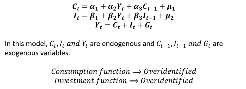
This is a complete model because it has 3 endogenous variables and 3 equations. It satisfies the condition that the number of equations must be equal to the number of endogenous variables. The third equation is simply an equilibrium equation, sometimes known as the identity equation. It contains no parameters and does not need to be estimated. Therefore, we need to estimate the consumption and investment functions.
This model contains 3 endogenous variables, but only 1 endogenous regressor. An endogenous regressor is an endogenous variable that appears on the right-hand side of equations. While consumption and investment are endogenous, they do not appear as regressors in any of the equations. Hence, income (Yt) is the only endogenous regressor in this model.
Step 2: check the identification of the model
Before estimating any simultaneous equation model, it is essential to check the identification of the model. This is because the method of estimation may depend on the identification of the model. Moreover, underidentified equations cannot be estimated. If an equation in the model is found to be underidentified, a different specification has to be used.
In our example, we have to determine whether the consumption and investment functions are identified or not. We can move on to estimation if the equations are exactly-identified or overidentified. We can use the Order and Rank Conditions to check the identification of the equations.
Underidentified – cannot be estimated
Just or Exactly-Identified – apply Indirect Least Squares (ILS)
Overidentified – apply 2SLS, 3SLS, LIML or FIML
Where 2SLS refers to Two-Stage Least Squares, 3SLS is Three-Stage Least Squares, LIML is Limited Information Maximum Likelihood and FIML refers to Full Information Maximum Likelihood.
The consumption and investment functions in our example are overidentified. We used the Order and Rank Conditions to determine that. We will not discuss the procedure of identification here because we have to focus on 2SLS and its estimation.
Because the equations are overidentified, we can apply 2SLS to estimate both the consumption and investment functions.
Step 3: apply Two-Stage least squares (2SLS) and estimate the overidentified equations
As the name Two-Stage Least Squares (2SLS) suggests, the estimation is carried out in two stages:
First Stage: estimate the Reduced-form equations
Second Stage: estimate the structural equations using first stage predictions as instruments
In the first stage, reduced-form equations are estimated. Reduced-form equations represent endogenous variables as a function of exogenous variables. That is, the endogenous variable is the dependent variable and exogenous variables are used as independent variables in the reduced-form equations.
In our example, we will estimate 1 reduced-form equation because only 1 variable (Income) appears as an endogenous regressor (on the right-hand side) in the model. The reduced-from equation for income (Yt) can be expressed as:
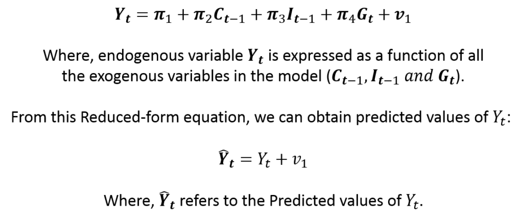
The results of the first stage, i.e. the predicted values of income (Yt), are used as instruments in the second stage. In the second stage, the consumption and investment functions are estimated separately using predicted values of income as instruments for the income variable. As a result, the following equations are estimated:
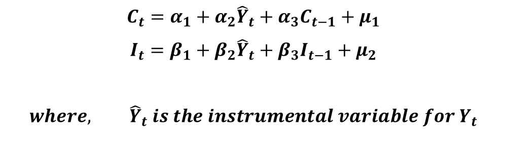
The results of these equations give us the 2SLS estimates. That is, the estimates from the second stage represent the structural coefficients of our consumption and investment functions. In practice, we do not need to estimate the two stages of 2SLS manually. Statistical software packages allow us to estimate the structural coefficients directly by taking care of both stages.
Let us look at the 2SLS results of our model:
Consumption Function
| 2SLS – Consumption | Observations = 62 | p > chi2 = 0.000 | ||
| R-square = 0.9998 | RMSE = 24076 | |||
| Variables | Coefficients | Standard Error | z | p-value |
| Yt | 0.2598118 | 0.0237767 | 10.93 | 0.000 |
| Ct-1 | 0.7124155 | 0.0398005 | 17.90 | 0.000 |
| Constant | 9200.814 | 3954.735 | 2.33 | 0.020 |
The above coefficients show the 2SLS estimates of the consumption equation. The interpretation of the coefficients is similar to that of OLS. Consumption is positively and significantly related to income. With a 1 unit increase in income, consumption increases by approximately 0.26. This coefficient can be interpreted as the marginal propensity to consume.
Additionally, consumption is significantly affected by past consumption. The inclusion of previous period consumption as an exogenous variable is similar to those in Habit Formation Models. This means that past consumption habits have a strong effect on current consumption as expected. This result is understandable as our consumption patterns stay more or less similar to our recent consumption habits. For instance, individuals who like coffee will consume some quantity of coffee in each time period as they are habitual to it.
Investment Function
| 2SLS – Investment | Observations = 62 | p > chi2 = 0.000 | ||
| R-square = 0.9958 | RMSE = 52322 | |||
| Variables | Coefficients | Standard Error | z | p-value |
| Yt | 0.0993128 | 0.0290062 | 3.42 | 0.001 |
| It-1 | 0.8243824 | 0.0934051 | 8.83 | 0.000 |
| Constant | -10094 | 8714.566 | -1.16 | 0.247 |
Similar to consumption, the investment is significantly dependent on income as well as previous period investment. The interpretation of coefficients is again similar. The constant, however, is insignificant here.
Important: Test of Overidentifying Restrictions revealed that the instrumental variables used in the investment function are not valid. This means that the results of the investment function are invalid as the equation has been misspecified. Therefore, we will have to make some changes to the specification of the model. In this example, we need to include past consumption (Ct-1) in the Investment function to eliminate the problem because this variable has been incorrectly excluded from the investment equation. We will discuss this problem in detail separately. Here, we will only focus on the procedure of estimating 2SLS.
Two-Stage least squares (2SLS) v/s OLS estimates
The Test of Endogeneity and Test of Overidentifying Restrictions were used to establish that the instrumental variables used in the consumption function were valid. Moreover, the income variable was observed to be endogenous. Go here to learn more about the application of the Test of Endogeneity.
Since Income is endogenous, the use of OLS is inappropriate and its estimates will be biased. The application of 2SLS gives us consistent estimates of the consumption function. The bias in the OLS estimates can be observed by comparing the estimated coefficients of the two models.
| Variables | 2SLS Coefficients | OLS coefficients |
| Yt | 0.2598118 | 0.298019 |
| Ct-1 | 0.7124155 | 0.6485614 |
| Constant | 9200.814 | 11902.91 |
By comparing the coefficients, we can observe that OLS overestimates the role of income and constant. And, it also underestimates the coefficient of previous period consumption. We know that the 2SLS coefficients are consistent because income is correctly treated as an endogenous variable, as shown by the Test of Endogeneity. However, OLS takes income as exogenous which leads to simultaneous equation bias. This is why some of the coefficients are overestimated and others are underestimated by OLS.