Robust Standard Errors and OLS Standard Errors

The Standard Error of an estimate is the measure of the standard deviation of that coefficient. It helps to determine the reliability or precision of a coefficient estimated by the model. Therefore, the smaller the standard error as compared to the value of the coefficient, the better the reliability. Here, we will discuss the theory, uses and implementation of OLS standard errors and Robust Standard Errors in detail.

For further details on the application of Ordinary Least Squares (OLS), see Ordinary Least Squares in Rstudio.

Econometrics Tutorials

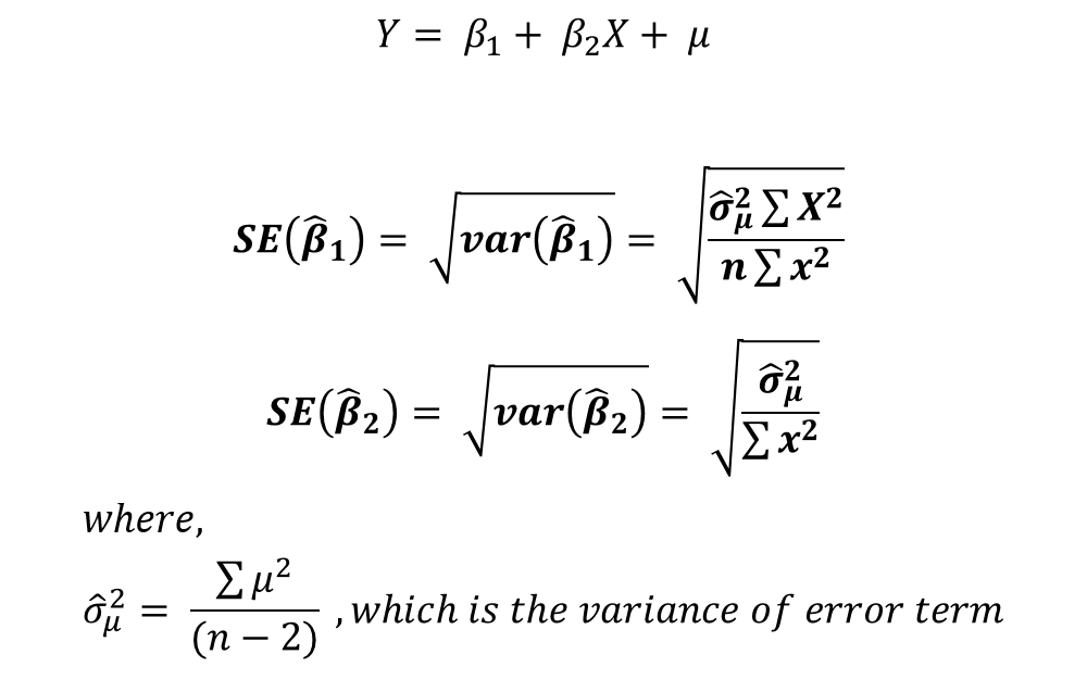
OLS Standard Errors in a two-variable model

In a two-variable model with one dependent and one independent variable, the standard error of intercept and slope coefficients can be estimated as follows:

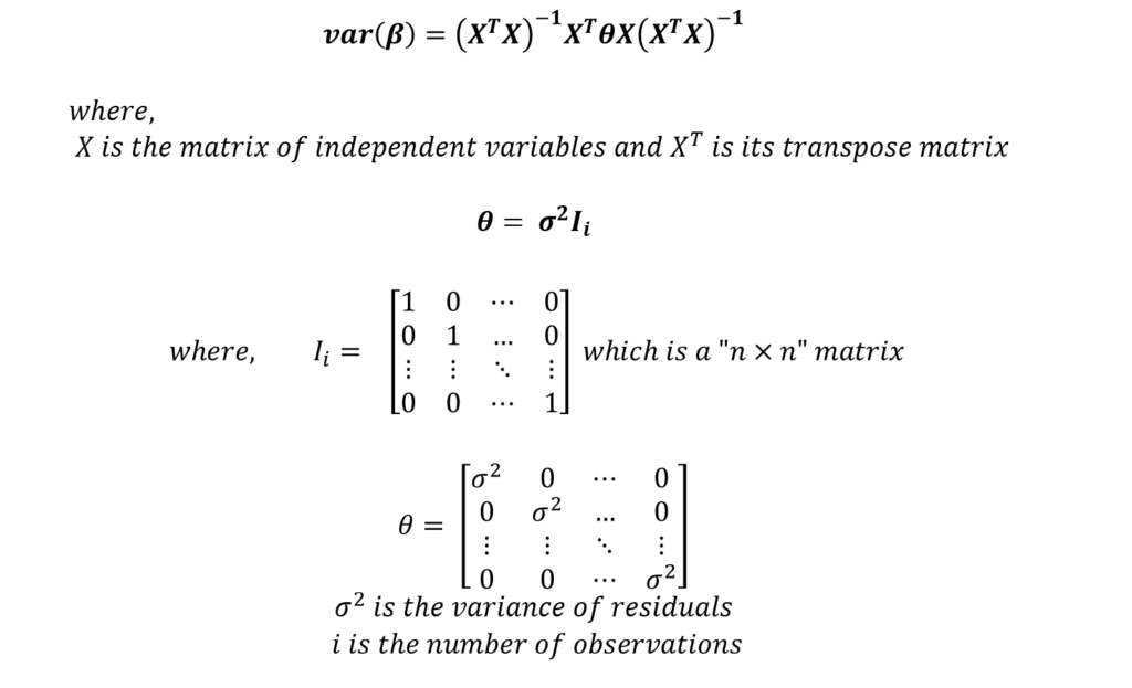
OLS Standard Errors in a Multivariate Model

In a multiple linear regression model, standard errors of coefficients can also be estimated using the matrix method:

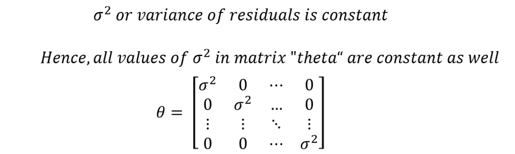
Assumption of Constant Variance in OLS Standard Errors

One of the assumptions of Ordinary Least Squares (OLS) is constant variance or homoscedasticity. This is also evident in the OLS standard errors.

In the above formula, the residual variance is constant because it is one of the assumptions of OLS. As a result, all the values of residual variance in the matrix “theta” are constant as well.

This further signifies the importance of the assumption of homoscedasticity in OLS. Furthermore, the calculation of Standard Errors is based entirely on this assumption.

Suppose, the model suffers from the problem of heteroscedasticity. Then, it will violate the assumption of constant variance. But, the OLS standard errors are still calculated with the assumption of homoscedasticity. Therefore, the OLS standard errors will not be reliable in the presence of heteroscedasticity.

Since the confidence intervals and P-values are estimated with the help of standard errors, the entire system of testing the significance of coefficients breaks down. The results will not be reliable because they are based on the assumption of constant variance. Whereas, the model suffers from heteroscedasticity or non-constant variance of residuals.

Heteroscedasticity and Robust Standard Errors

With heteroscedasticity or non-constant variance of residuals, the OLS standard errors are no longer reliable. One of the solutions to this problem is the use of Robust Standard Errors.

Robust Standard Errors are also known as White’s Heteroscedasticity Consistent Standard Errors. The Robust Standard Errors incorporate non-constant variance into the formula of standard errors. As a result, the assumption of constant variance is dropped from the standard errors and we can account for heteroscedasticity.

To adapt to heteroscedasticity, the matrix “theta” in the standard error formula is then replaced by a new matrix. Let us take a look at different ways to account for heteroscedasticity:

HC1 Robust Standard Errors

The matrix “theta” is replaced by another matrix to include non-constant variance as follows:

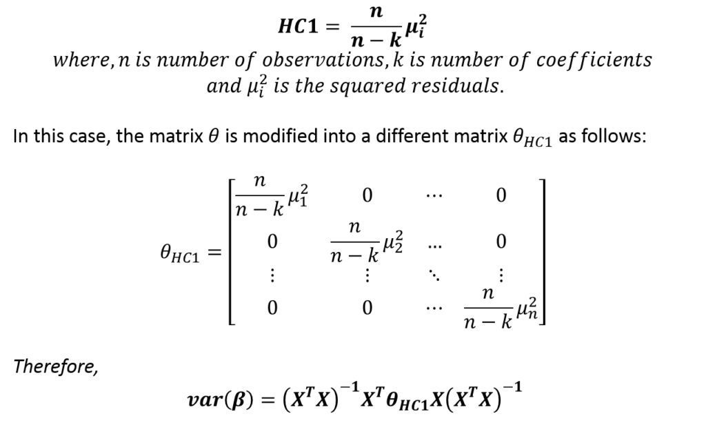
All the diagonal elements in the new matrix “theta_HC1” are different. Hence, the HC1 Robust Standard Errors are based on non-constant variance.

HC3 Robust Standard Errors

HC3 robust standard errors are the most widely used and generally considered the best standard errors in the presence of heteroscedasticity. These are estimated as follows:

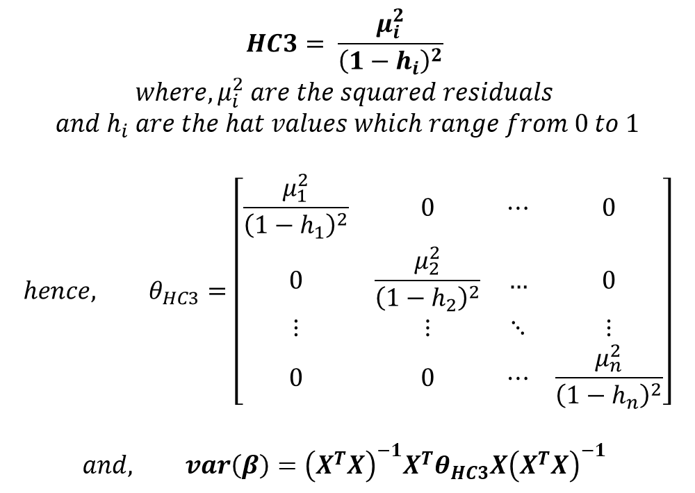
The calculation of “hat values” and, therefore, HC3 robust standard errors can be complex. However, statistical software packages make their implementation easy.

Implementation

To illustrate the use of standard errors, we will apply OLS to a model with the problem of heteroscedasticity. Furthermore, we will estimate OLS standard errors and Robust Standard Errors (HC3) for the model and compare the results.

The “Rent” of apartments is the dependent variable of the model. The rent is determined by the “Number of rooms” and also the presence of “Central Heating” in the apartment. The independent variable of central heating is a categorical variable with the value of “1” for apartments with central heating and, hence, “0” for apartments without central heating.

OLS Standard Errors

The results of the model with OLS standard errors are:

			R-square = 0.8427
Rent
	Coefficient	Standard error	t	p-value
Rooms	2.258247	0.2374286	9.51	0.000
Heating	1.514989	0.699378	2.17	0.045
Constant	7.780602	0.9339954	8.33	0.000

Robust Standard Errors

This model suffers from heteroscedasticity, therefore, OLS standard errors are not reliable. Hence, we estimate the model with Robust Standard Errors (HC3).

			R-square = 0.8427
Rent
	Coefficient	Robust HC3 Standard error	t	p-value
Rooms	2.258247	0.2839767	7.95	0.000
Heating	1.514989	0.6445046	2.35	0.031
Constant	7.780602	0.7476062	10.41	0.000

From the above results, it is evident that the value of coefficients remains the same, but, the estimated value of standard errors and the resultant “t” and “p-values” are different.

The OLS standard errors were under-estimating the standard error for the coefficient of “rooms”. On the other hand, it was over-estimating the standard errors of the constant and the coefficient of “heating”.

The coefficients, on the other hand, are significant because the P-values are less than 0.05. We can conclude that heteroscedasticity is not a serious problem in this case because there is no change in the significance of coefficients. They were statistically significant with OLS standard errors and are still statistically significant with Robust Standard Errors.

Note: in the presence of heteroscedasticity, it is best to use HC3 Robust standard errors. Even if heteroscedasticity is not detected, it is advisable to report Robust standard errors along with OLS standard errors in every model to ensure heteroscedasticity is not a problem. It is considered a good practice to report both standard errors.

Econometrics Tutorials