Ordinal utility analysis and indifference curves were developed to overcome the shortcomings of the cardinal utility analysis, which is based on the unrealistic assumption that utility can be accurately measured or assigned a value. For instance, there is no reasonable way to tell how many units of satisfaction a consumer derives from a product.
To address this problem, ordinal utility analysis is based on the idea that utility cannot be measured, but, it can be ranked. In other words, consumers can rank different goods based on their preferences. For instance, if faced with a choice between two goods, consumers know which good they prefer more and will buy that product. Hence, consumer equilibrium is dictated by the ranking or ordering of preferences. They are aware of the product that they prefer the most, which gives them the highest satisfaction.
For example, a consumer can tell whether he or she prefers a cupcake or a muffin. Similarly, choices can also be ranked among different combinations or bundles of goods. For instance, a consumer can tell whether he or she prefers to consume a pizza with a soda, a burger with a shake or any other combination.
Econometrics Tutorials with Certificates

Assumptions
- Completeness: this implies that preferences are complete, i.e. consumer can rank all products by comparing them. For instance, while comparing two goods or combinations X and Y, a consumer either prefers X or prefers Y or has equal preference.
- Transitivity: suppose a consumer prefers good X over Y and prefers good Y over Z. Then, it is automatically implied that the consumer prefers good X over Z.
- More is better: it is assumed that consumers do not feel satiated and always prefer more. If a combination X has more of a good as compared to the other combination Y, then combination X will be preferred.
Consumer equilibrium under ordinal utility analysis can be understood with help of indifference curves and budget lines. It is often referred to as indifference curve analysis.
Indifference Curves
An indifference curve shows various combinations of two goods that give the same total satisfaction or utility to a consumer. This implies that the consumer has the same preference for all the combinations of two goods on the indifference curve. Therefore, he or she will feel indifferent about which combination to buy.
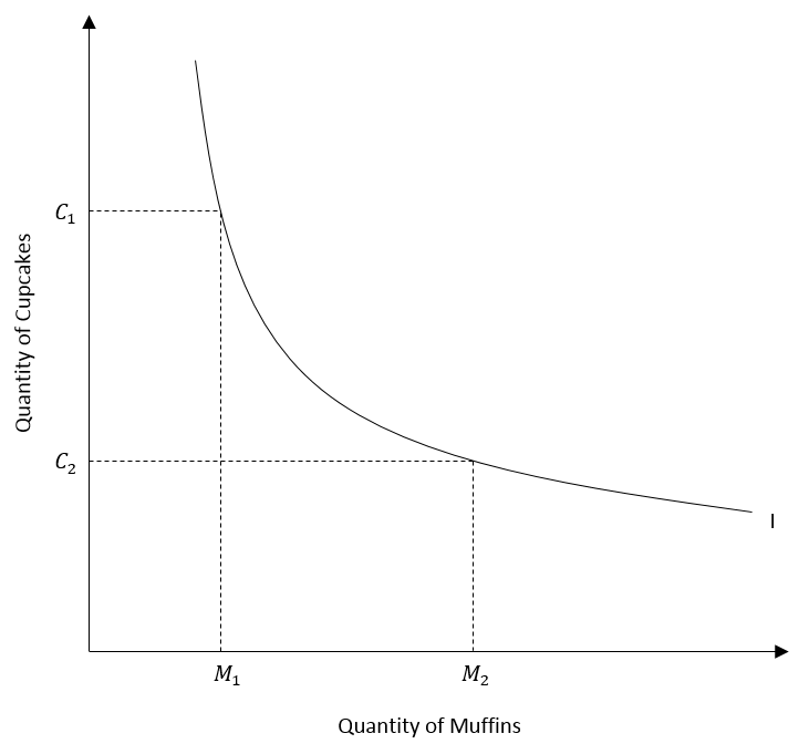
In the diagram, an individual consumes more cupcakes than muffins in one combination and more muffins than cupcakes in another combination. However, the satisfaction or utility derived from both combinations is the same. The consumer will be indifferent between the two.
Therefore, the indifference curve in the diagram shows the various combinations of cupcakes and muffins that give the same satisfaction to the consumer.
Indifference map from indifference curves
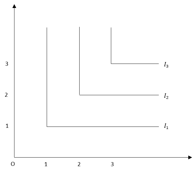
An indifference map consists of a number of indifference curves associated with two goods. It shows different levels of total utility or satisfaction from different combinations of two goods. Each indifference curve depicts a different level of total satisfaction. They do not intersect each other because the level of satisfaction is different on each curve.
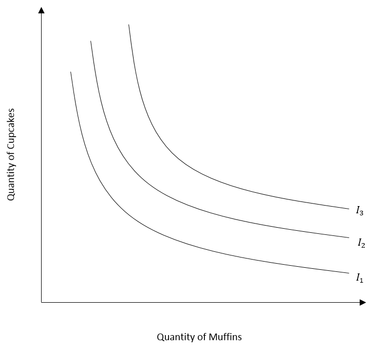
The level of total satisfaction or utility derived increases with movement towards the right and decreases with movement towards the left of the indifference map. In the diagram, the indifference curve I3 represents a higher level of utility as compared to I2 and I1. The indifference curve I1 has the lowest utility among the three indifference curves.
Slope of Indifference Curves
Indifference curves are downward sloping because of the trade-off between two goods. If a consumer gets more quantity of one good, their total utility will increase. However, an indifference curve represents the same level of utility. To maintain that same level of utility on a given indifference curve, the quantity of the other good must be decreased to offset the increase in utility.
Hence, there is a trade-off where more of one good means less of the other good on an indifference curve. Since one good is substituted for the other, both their quantities are inversely or negatively related. Hence, indifference curves end up being downward sloping.
Marginal Rate of Substitution (MRS)
The marginal rate of substitution (MRS) is a measure of the trade-off between two goods or bundles on an indifference curve. It can be defined as the quantity of good A that a consumer is willing to give up for an additional unit of good B. The slope of the curve at any point on the indifference curve is its MRS at that point.
For example, if the slope is 2 (ignoring the negative sign), MRS will be 2 at that point. The consumer will be willing to forego or give up 2 units of good A to get an extra unit of good B.

Note: we ignore the negative sign because the consumer is giving up some quantity of good A. Therefore, MRS will always be negative because the change in the quantity of good A is negative. As the indifference curves involve a trade-off between goods and are downward sloping, their slope is always negative. Hence, we focus on the magnitude by taking the absolute value of the slope.
Convexity of Indifference curves and diminishing MRS
One of the most important features of indifference curves is diminishing MRS, which is the reason why indifference curves are convex to the origin. Diminishing MRS represents an important insight into consumer preferences.
As consumers obtain more and more of a good, their preference for that good keeps decreasing. Hence, they will be willing to forego less and less of the other good to obtain an additional unit. For instance, as consumers get more of good B, they will be willing to give up lesser and lesser of good A to get an additional unit of good B. As a result, MRS will go on diminishing along the curve.
In other words, the slope of the indifference curve becomes less and less negative with more quantity of good B. The magnitude of slope (absolute value) will keep decreasing. Hence, MRS will keep decreasing with more of good B.
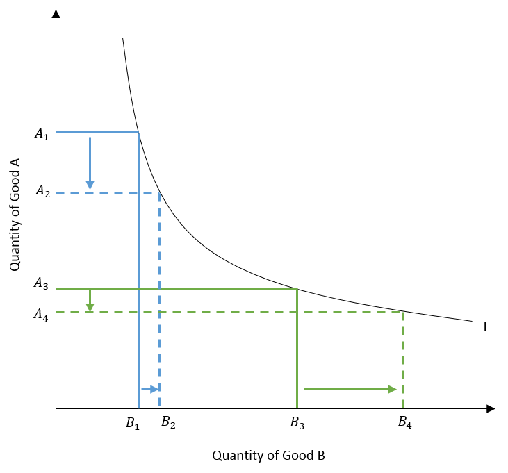
In the diagram, it can be observed that MRS is initially high, and goes on declining with more quantity of B obtained. Initially, as quantity increases from B1 to B2, the consumer is willing to give up a lot of good A (A1 to A2). It implies that MRS is high in the earlier portion of the indifference curve. As we move along the curve, the consumer is willing to give up a lot less of good A (A3 to A4) for additional quantities of good B (B3 to B4). Hence, MRS is diminishing as more of good B is obtained.

Exceptional Cases of Indifference Curves
Perfect Substitutes
In the case of perfect substitutes, the MRS is constant and the slope of the indifference curve is always constant as well.
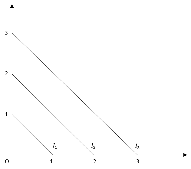
MRS = 1 and remains constant at 1
In the diagram, we assume that tea and coffee are perfect substitutes for a consumer. The consumer is completely indifferent between good A (coffee) and good B (tea). Therefore, he or she will either have a cup of coffee or a cup of tea. As a result, the consumer will be willing to give up 1 cup of coffee for an additional cup of tea.
Note: for perfect substitutes, MRS needs to be constant, but it does not have to be 1. The slope and MRS can be any constant value. For instance, MRS can be constant at 2 where consumers will be completely indifferent and willing to give up 2 units of good A for an additional unit of good B.
Perfect Compliments
The MRS is infinity whenever the consumer has more of good B. MRS is zero when the consumer has more of good A as compared to B. Since the goods are perfect compliments, utility cannot be increased by obtaining just one good. It can only be increased by purchasing both goods.
More left socks (Good A) means MRS = infinity
More right socks (Good B) means MRS = 0
In the example, consumers will buy both left and right socks to increase utility. Utility cannot be increased by buying only a left or a right sock. If the consumer has extra left socks, MRS is infinite. The consumer will give up left socks to obtain more right socks. Conversely, if the consumer has extra right socks, MRS is zero because the consumer will not buy more right socks.
Budget constraint and Budget Line
Consumer choices are dictated not just by preferences and utility, but also by the income or budget of the consumer. Consumers always want more of a commodity for higher utility. But, budget acts as a constraint beyond which a consumer cannot spend to purchase goods. Therefore, their choices are dependent on the amount of budget (income/purchasing power) available.
Suppose, a consumer has a budget of ‘Y’ to be spent on two goods, good A and good B. Then, the budget constraint can be specified as:
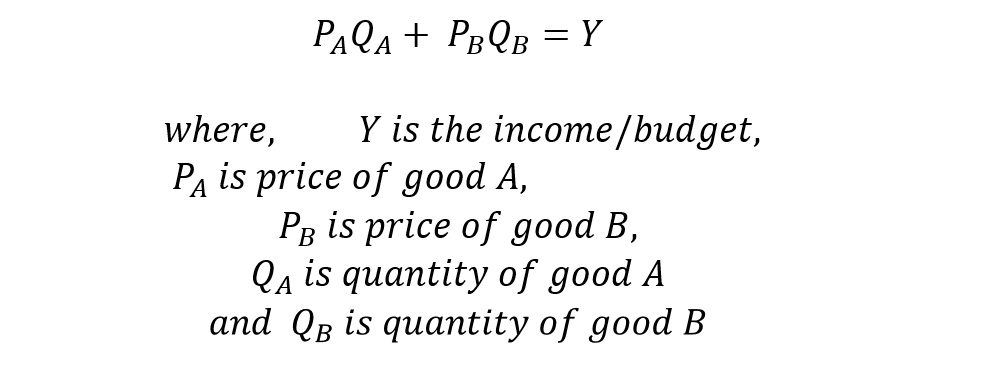
PAQA will be the amount of money spent on good A and PBQB will be the amount of money spent on good B. According to the constraint, the sum of money spent on both goods will be equal to Y, which is the budget.
Budget Line
The budget line can be derived with help of budget constraint. The budget line represents the various combinations of goods that can be bought with the given income or budget of the consumer. It is assumed that there are no savings and the consumer spends entire income on two goods.
Let us consider an example where the income of the consumer is $100, the price of good A is $1 and the price of good B is $2. If the consumer buys only good A, then the entire income of $100 will be used to purchase 100 units of good A. If the consumer decides to buy only good B, then $100 will be used to buy 50 units of good B. The budget constraint can be used to calculate various combinations of goods A and B that can be purchased:
PAQA + PBQB = Y
1(QA ) + 2(QB)= 100
| Quantity of good A | Quantity of good B | Total money spent |
| 0 | 50 | 100 |
| 20 | 40 | 100 |
| 40 | 30 | 100 |
| 50 | 25 | 100 |
| 60 | 20 | 100 |
| 80 | 10 | 100 |
| 100 | 0 | 100 |
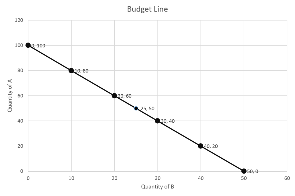
In the diagram, the line represents the budget line with different combinations of A and B. The slope of the budget line can be expressed as follows:
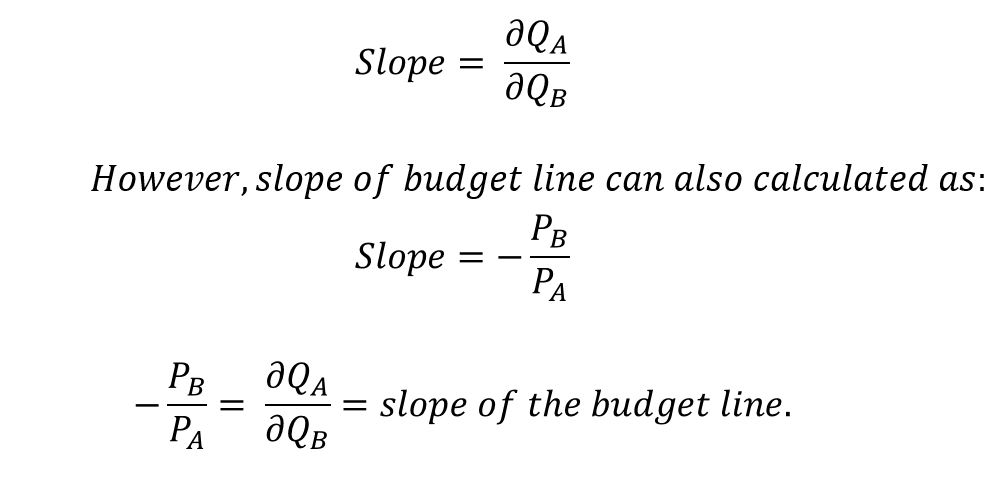
In our example, the slope of the budget line is -2.
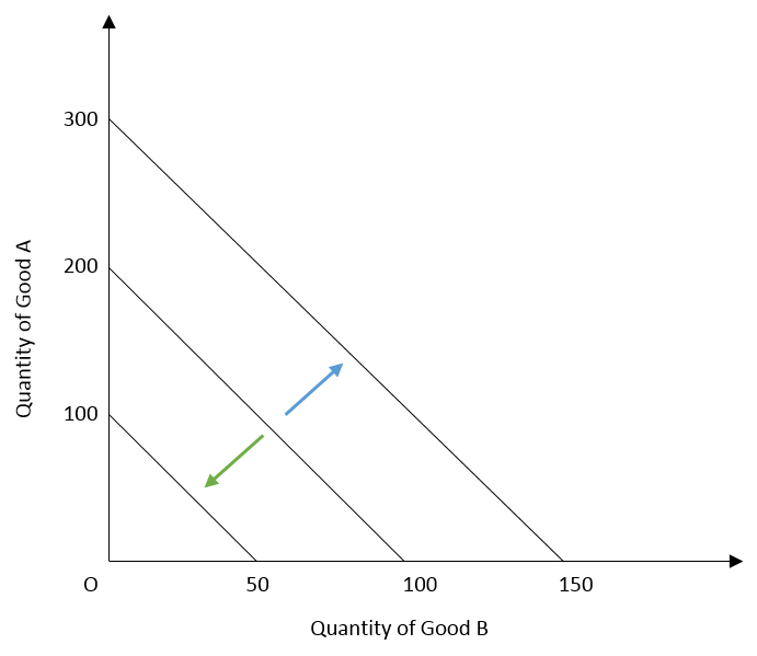
Changes in Budget Line
- Changes in income: budget line will shift upwards with an increase in the income of consumer and shift downwards with a decrease in the income of consumer. As income rises, consumers can purchase more quantities of both goods which shifts the budget line upward. Because the prices of both goods remain the same, the slope of the budget line does not change.
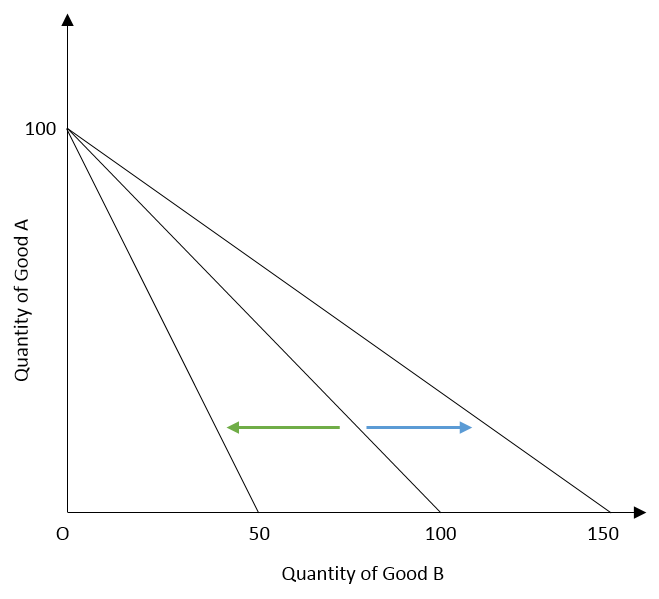
- Changes in price of goods: if the price of one of the goods changes, it leads to a rotation of the budget line. In such a case, the slope of the budget line changes. For instance, if the price of good B decreases, then the budget line will rotate in the rightward direction. The intercept associated with good B will rotate to the right on the x-axis. This happens because the consumer can now buy more of good B with a fall in its price. If the price of good B rises, consumers will be able to buy less of good B. Then, the budget line will rotate to the left. In this case, the slope of budget line will increase as it becomes steeper.
Consumer Equilibrium and Choice under Indifference Curve Analysis
Consumers aim to maximize their satisfaction with the given amount of income. Consumer equilibrium will be achieved at the combination of two goods which gives the highest utility with the given budget. This equilibrium will occur at the point where the budget line is tangent to the indifference curve. At this point, the slope of the budget line and indifference curve will be equal.

Note: slopes of both the budget line and indifference curve are negative because they are downward sloping. Here, we are concerned about the magnitude of the slopes which should be equal. Therefore, the negative signs can be ignored because it simply implies that both are sloping downwards.
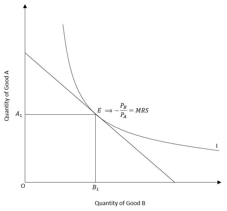
Point E shows the tangency of the budget line with the indifference curve. Hence, E is the point of equilibrium where the slopes of the indifference curve and budget line are equal. At equilibrium, the consumer will purchase A1 quantity of good A by allocating PAA1 amount of income on good A. The remaining income PBB1 is allocated to purchase B1 quantity of good B. This combination of good A and good B maximizes the utility of the consumer.
Why is consumer equilibrium at point E (point of tangency)?
We can illustrate that E is maximizing utility at the given income and prices of A and B. To do this, we will consider different points associated with various combinations of good A and good B.
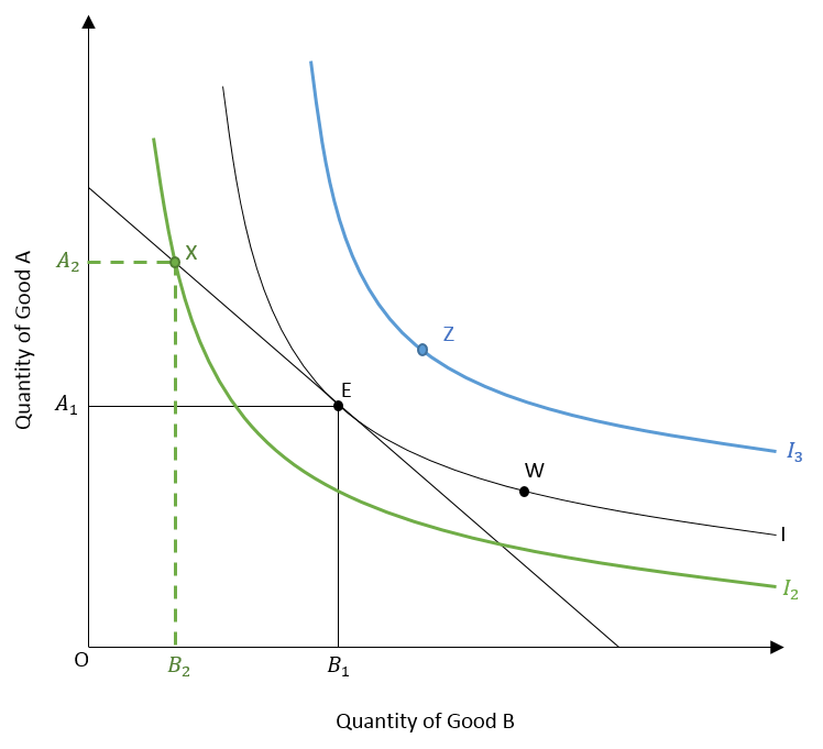
At W
Point W gives the same utility as equilibrium point E because they are on the same indifference curve (I). However, the combination of goods A and B at this point is not affordable to the consumer as it lies beyond the budget line, The consumer cannot purchase that combination of quantities of A and B. In other words, the consumer is getting the same level of utility at point E by spending within his or her budget. He/she will not spend more to get to point W for the same level of utility.
At X
Point X lies on the budget line and the consumer will purchase the combination of A2 and B2 quantity of goods A and B respectively. But, this point X lies on indifference curve I2, which is associated with a lower utility level as compared to the indifference curve of point E. Even though consumer can afford to be at X, he/she will not be at the maximum utility. This is because the utility can be increased by shifting to “I” and equilibrium point E.
At Z
Point Z is on indifference curve I3 with the highest level of utility. However, the consumer cannot afford that combination because of limited income as point Z lies beyond the budget line. The consumer can operate at point Z if the income increases and the budget line shifts upward. Or, if there is a huge drop in the price of good B or good A and the budget line may rotate towards point Z. With given income and prices, however, point E gives maximum utility where the consumer will be at equilibrium. He/she will have no incentive to change this combination of good A and good B.
Marginal Utility, MRS and Law of Equi-marginal Utility
Marginal utility refers to the satisfaction gained from the consumption of one additional unit of a commodity. Total utility is the sum of marginal utilities gained from each successive unit consumed. The law of diminishing marginal utility states that as more of a commodity is consumed, the additional satisfaction from each successive unit goes on decreasing.
The logic behind this concept is that as a consumer gets more of a commodity, his or her want for that commodity and the resultant satisfaction from it will decrease. For example, the marginal utility from getting the first car will be high. Buying an additional car will not yield the same level of utility.
Relationship between Marginal Utility and MRS
As the consumer buys more of good B, he or she will gain some marginal utility from the purchase of one additional unit. Suppose, this increase in the quantity of good B yields an extra utility of MUB per unit. However, the consumer also has to give up some quantity of good A to obtain that additional good B. This fall in the quantity of good A also leads to a fall in utility due to less consumption. Let this reduction in utility be denoted by MUA per unit.
However, an indifference curve has the same level of utility throughout. Hence, the total utility lost due to a fall in good A will be equal to the total utility gained from extra units of good B. In other words, the sum of both will be zero because the total utility has to remain the same along the indifference curve.
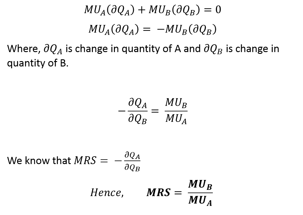
This shows that MRS is the ratio of the marginal utility of good B and the marginal utility of good A. As the law of diminishing marginal utility operates, the numerator (MUB) falls because the quantity of good B is increasing. This leads to diminishing marginal utility of B. On the other hand, the denominator (MUA) will increase as less good A is consumed. This is because its marginal utility will be high with less quantity consumed.
As a result, MRS will keep decreasing with movement along the indifference curve. This further proves the existence of diminishing MRS. Furthermore, the marginal utility gained from extra units of good B can be considered as the marginal benefit. Whereas, the quantity of good A that the consumer has given up is considered as marginal cost.
The principle of Equi-marginal Utility
We also know that consumer equilibrium is achieved when MRS is equal to the ratio of prices of goods:
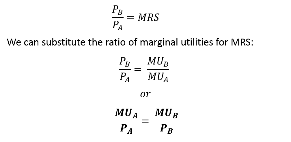
Therefore, we can conclude that utility is maximized when the ratios of marginal utility to price for each good is the same. This also implies that marginal utility per unit (dollar) of expenditure on each good is equal. This makes sense because a consumer will allocate income towards the commodity that gives more marginal utility.
As consumer buys more of a good, it will also reduce the marginal utility from the next unit of that good. This will go on till the marginal utility per unit (dollar) of expenditure becomes the same for all the goods concerned. That is, the last dollar spent on each good yields the same marginal utility. This is also known as the principle of Equi-marginal utility.
Econometrics Tutorials with Certificates

This website contains affiliate links. When you make a purchase through these links, we may earn a commission at no additional cost to you.
very helpful, thanks a ton!
You’re welcome!