Impulse Response Functions or IRFs are used to study the effects of shocks or impulses in a VAR or VECM system. It traces out one unit or one standard deviation shock to an endogenous variable and its effects on all the endogenous variables in a VAR or VECM, keeping all other variables and shocks constant.
For instance, consider a VAR system with income, consumption and investment as endogenous variables. Using impulse response functions, we can deliver one standard deviation or one unit shock to income. The effects of that shock can be seen in all the endogenous variables and equations of that VAR model. Hence, we can analyse the effects of income shock on consumption and investment behaviour over different time periods.
Impulse Response Functions are the most important application of VAR and VECM models. They are useful in understanding the dynamic behaviour of variables in a system. Furthermore, IRFs are important tools in predicting the effects of impulses/shocks and policy analysis.


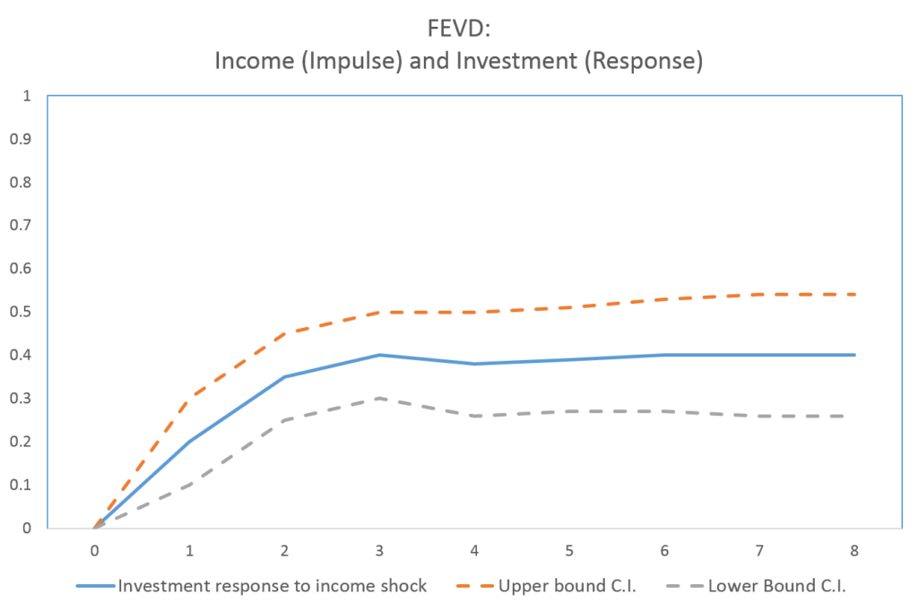
Vector Autoregression (VAR) specification: Reduced-Form VAR
Suppose, we have a VAR model of order 2 or VAR(2):
This model contains 3 endogenous variables. Each equation has 2 lags of income, consumption and investment as independent variables. The choice of lags or lag length can be made using various Information Criteria.
This model is known as a Reduced-Form VAR because the endogenous variables are determined only by their past values and the past values of other variables. This implies that no endogenous variable affects another in the same time period, i.e. there are no contemporaneous effects.
The error terms in a VAR system are referred to as impulses or innovations. Additionally, the shocks or impulses to an endogenous variable are introduced through these error terms. Suppose, we wish to study the effects of income shock on the above VAR system. The shock is introduced in the 1st equation of income through its error term u1t.
The shock or impulse and its effects can be traced using IRFs as follows:
Impulse Response Functions (IRF)
IRFs can be easily estimated using statistical software packages. Let us assume a one unit shock to income. The shock will affect income (1st equation) in the same time period. However, the effects of that shock will be visible on other endogenous variables in the next time period. This happens because our VAR(2) system contains only the lags of variables, i.e. endogenous variables are explained by the previous 2-period lags. There are no contemporaneous effects or variables are not explained by the current period values.
Therefore, as the shock or impulse occurs, its effect on income will be seen in the same time period because it is an income shock. However, its effects on consumption and investment can be observed from the next time period onwards.
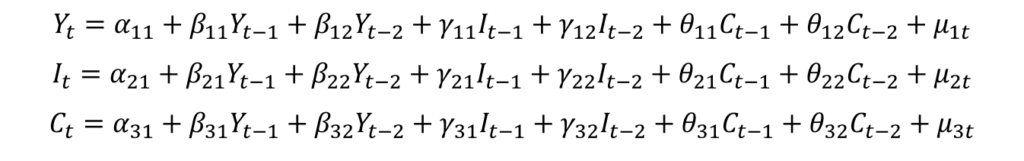
Effect of Income Shock on Investment
The graph shows that investment does not respond to income shock in the same time period. However, there is a positive relationship between income and investment. One unit positive shock to income leads to a 0.4 unit increase in investment in the first time period after the shock. In time period 2, the shock further causes a 0.5 unit increase in investment. The effects of the shock start to reduce in the third time period and the impulse response function converges to zero. Finally, the effects of the shock die out in time period 5, where the lower bound confidence interval is zero.
Additionally, the upper and lower bound confidence intervals show a range within which the impulse response may vary. The effects of the shock are significant in 5 time periods as confidence intervals are well above zero. Hence, we can say that any shock to income will have a positive impact on investment, other things remain constant. Moreover, the effects of the shock will be significant and persist for 5 time periods after the shock occurs.
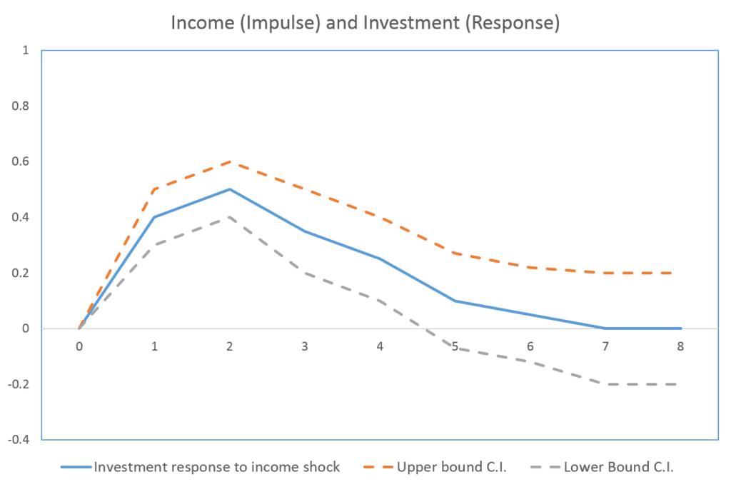
Effect of Income Shock on Consumption
Similar to investment, we can observe a positive relationship between income and consumption. One unit increase in income due to shock leads to a 0.6 unit increase in consumption. The effects of the shock are less in the second time period. Moreover, the impulse response function converges to zero in the third time period as the effects of the shock die out.
As compared to consumption, the effects of income shock last longer on investment. Whereas, the effects fall to zero quickly in the case of consumption.
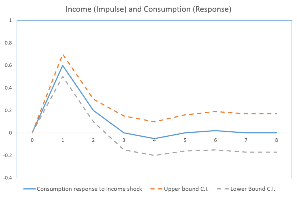
Forecast Error Variance Decomposition (FEVD)
In addition to IRFs, we also have the option to estimate Forecast Error Variance Decompositions (FEVD). FEVD shows the proportion of variations in an endogenous variable that is explained by a shock or impulse.
In the above example, we focussed on income shock and its effects on investment and consumption. Along with IRFs, we can obtain FEVD. For instance, FEVD for income shock on investment will show the proportion of variation in investment that is explained by income shock.
In this FEVD, we can observe that approximately 20% of the variations in investment are explained by income shock in the first time period. As we move further to the next time periods, the proportion of variation in investment explained by income shock goes on increasing. By time period 3, around 40% of the variations are explained by income shock. This proportion stabilises at approximately 40% beyond time period 3. The remaining variations in investment (unexplained by income shock) are explained by other shocks- consumption and investment shocks.
Similarly, we can construct FEVDs for investment in response to consumption shocks or investment shocks. These shocks explain the remaining proportion of variations in investment. Finally for consumption shocks, we will see the proportion of variation in investment explained by consumption shock. Such analysis helps us decompose the effects of various shocks and trace those effects over time.
Orthogonalized Impulse Response Functions (OIRFs) and SVAR
Orthogonalized-IRFs (OIRF) allow us to include contemporaneous effects of shocks or impulses. This means that we can use OIRFs to include the effects of shocks on endogenous variables in the same time period.
In the IRFs above, the income shocks affected investment and consumption in the next time period. This happened because we used a Reduced-Form VAR, where we included only past values of variables as independent variables in each equation. In reality, however, income could affect consumption and investment in the current time period as well. That is, any changes or shocks to income in the first equation will have an effect on investment and consumption in the same time period. Further, such a VAR model which includes contemporaneous effects can be stated as follows:
Structural-VAR or SVAR

This model including contemporaneous effects is a simplified insight into the Structural VAR or SVAR. It allows us to include more information in the model as compared to a Reduced-Form VAR because we have included current period variables in the model.
The first equation of income is similar to that of the Reduced-Form VAR as income is explained only by past or lagged values. The second equation for investment, however, contains contemporaneous effects of income on investment along with lagged or last values. The current period income affects investment instantly, i.e. in the same time period. Hence, the effects of any shocks to income will be observed on investment in the same time period.
Similarly, consumption is affected by income and investment in the same time period. Any shock to income or investment affects consumption in the same time period.
NOTE: we cannot include contemporaneous effects in all the equations because of the problem of Identification in simultaneous equation models. Hence, our model includes current period income to explain investment (2nd equation) and current period income and investment to explain consumption (3rd equation). The first equation of income does not include any current period variables. This type of structure is referred to as “Cholesky Decomposition”. This makes our SVAR model Exactly Identified.
OIRFs (orthogonalized impulse response functions)
OIRFs are estimated after incorporating contemporaneous effects in the model. They give more information as compared to simple IRFs because they include current period effects as well.
Important: the ordering of variables has an impact on OIRFs. In our example, we have ordered our variables as income, investment and consumption. This implies that income will not be affected by other endogenous variables in the current time period. Consumption, on the other hand, is affected by both income and investment contemporaneously but does not have any effect on other variables in the current time period. Therefore, the ordering of variables determines which variables will affect others in the current time period. Finally, this decision must be based on some economic theory or relevant economic considerations.
Interpreting OIRFs (orthogonalized impulse response functions)
The interpretation of OIRFs is similar to IRFs. Let us take a look at some examples:
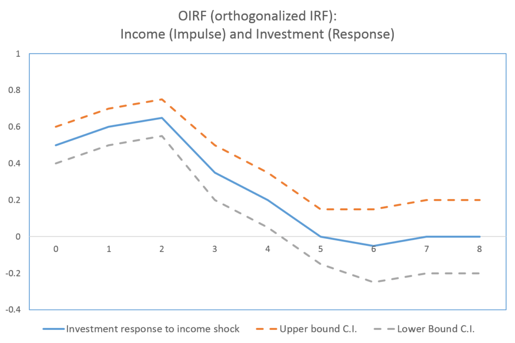
In the SVAR model and our ordering of variables, income affects investment contemporaneously. As a result, one unit positive shock to income increases investment by approximately 0.5 units in the current time period or instantly. The effects of the shock increase in the first and second time period after the shock and start declining after. The effects of the shock converge to zero in the fifth time period. Therefore, we can conclude that income has a positive and significant impact on investment. Moreover, the effects of any shock to income will persist on investment for 5 time periods in the future.
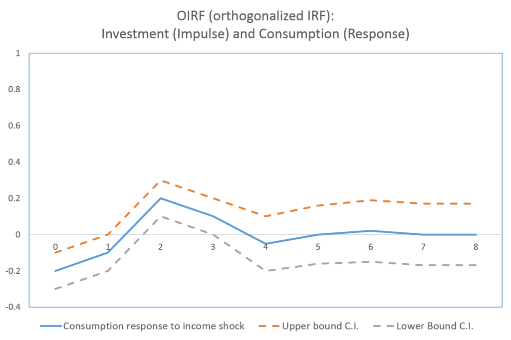
Based on the ordering of our variables, investment affects consumption in the same time period. It is evident from the above OIRF as a positive shock to investment reduces consumption in the current time period. The OIRF shows that one unit positive shock to investment will decrease current consumption by 0.2 units. This negative effect is reduced in the first time period. In the second time period, we can observe that investment shock has a delayed positive impact on consumption. This means that positive investment shocks will initially reduce consumption in the current period, whereas, they will have a delayed positive impact on consumption after two time periods.
Reliability of Impulse Response Functions
VAR
Before estimating IRFs, OIRFs or FEVDs from VAR or SVAR model, we must ensure that:
- the endogenous variables in the VAR/SVAR model are stationary. If the variables are not stationary, the results of the model will not be reliable and we should not implement IRFs. Hence, we must determine the order of integration of variables before estimating VAR/SVAR. If the variables are level stationary or I(0), we can apply VAR to the original variables. If variables are integrated of order 1 or I(1), we may prefer VAR after transforming the variables in their first deference form.
- VAR/SVAR model is stable. A stability check is necessary to avoid exploding forecasts or exploding IRFs. If the VAR model is stable, the IRFs will converge to zero after some time periods. If the VAR model is unstable, the IRFs will explode and will not be reliable. This happens when the variables are non-stationary and are not transformed appropriately.
- the model does not suffer from autocorrelation. If we detect autocorrelation, we must include more lagged variables in the model. Furthermore, the choice of lag length must ensure that autocorrelation is eliminated from the model.
The tests of stationarity, stability of VAR and autocorrelation test after VAR can be easily performed using statistical software packages.
Note: In a stationary VAR, the IRFs and OIRFs must converge to zero after some time periods. If they do not converge back to zero, the VAR model is not stable and reliable.
VECM
Similar to VAR, we must check for autocorrelation and the stability of the VECM model. The VECM is applied in the presence of cointegration. As a result, we obtain both short-run and long-run coefficients from the model.
In VAR, the effects of shocks or impulses always converge to zero after some time periods. But, this is not the case for VECM models. The IRFs or effects of the shocks may or may not converge to zero in a VECM model. Hence, we have two different types of shocks or impulses in a VECM model:
- Transitory shocks: when the IRFs or OIRFs converge to zero after some time periods, they are known as transitory shocks. The effects of these shocks die out after some time. For example, the effect of an income shock on consumption may become zero after a few time periods and it will not permanently increase consumption.
- Permanent shocks: the IRFs or OIRFs do not converge to zero in the case of permanent shocks. Instead, they stabilize around a positive or negative value. Such shocks have a permanent effect on the response variable. For instance, an income shock may permanently shift investment upwards.
Econometrics Tutorials with Certificates


This website contains affiliate links. When you make a purchase through these links, we may earn a commission at no additional cost to you.
Thanks
Welcome!!
Nice!! But, is Impulse response a must after VECM? What if VECM long-run variables are significant; however, the impulse response is not significant at all?
Impulse responses being insignificant does not imply that there is no effect. It simply means that the results of impulse responses are inconclusive. They may be insignificant due to reasons such as insufficient data. In these cases, a lot depends on the objectives of your study. It is not a must to estimate the impulse responses after VECM.
Hi, maybe you can help me. I chose to do VECM model regarding cointegration between variables I(1). But I also added to my VECM model exogenous variables, but I can’t a way to plot IRF, because IRF function takes only those variables which were cointegrated. Is it somehow possible to add exogenous variables as well? I am using R
Hello. The “MTS” and “lpirfs” packages provide functions to include exogenous variables in IRFs for VAR models. The MTS has a function “VARXirf” and lpirfs has a function “lp_lin” that allow exogenous variables to be included for IRFs. You can look into these packages and check whether these will work for your model. I don’t think a similar function is available for VECM. Depending on your research objective, maybe you can convert your VECM into VAR and proceed with IRFs.
Dear sir,
Can you give me the name of any paper discussing this issue?
Thank you very much!
Dear sir,
Can you give me the name of any paper discussing this issue?
Thank you very much!
There are several good research papers and books related to Impulse Response Functions. If you can tell me more about the exact issues or questions you have related to IRFs, I can suggest some useful readings.
good work and great insights. allow me to ask what to do when you using a VECM Model and one the variable becomes stationery at second order?
It is common to encounter variables that have different orders of integration. For example, you might have a variable that is stationary at first difference or I(1) and another variable that is stationary at level or I(0). If variables are integrated at different orders like this, you might be better off using the Autoregressive Distributed Lag (ARDL) approach instead of VECM. ARDL allows variables at different orders of integration and you can include an error correction term in the model. A disadvantage of the ARDL approach is that you cannot have more than one cointegrating relationship in the model or I(2) variables. In case of a mix of I(2) variables with I(0) or I(1) variables, you may have to resort to Toda-Yamamoto approach.
Thanks much,,, that is to mean that the cointegration rank for an ARDL must always be 1. I did apply ARDL Bound Test for cointegration and the F-statitisc is greater than the Upper Bound, meaning there is cointegration justifying the adoption of VECM . however i was stuck on determining the number of cointegration ranks in this case
Welcome. If you suspect multiple cointegrating vectors or relationships, you can use Johansen’s approach or Johansen’s Cointegration test. It will also help you in determining the specification of your VECM.
Virenrehal, your insights have been helpful to me a lot, am so grateful.Allow me to seek your assistance once more, am stuck on the interpretation of the vecm results and also on performing IRFs. Kindly assist
Thank you for your kind words and appreciation. Please take a look at the post on VECM Estimation and Interpretation. It provides a detailed understanding of the results of VECM and might be helpful to you. Here is the link: https://spureconomics.com/vecm-estimation-and-interpretation/
Please feel free to ask any specific questions you may have about VECM and IRFs. If you wish, you can also contact me using E-mail or WhatsApp. The information is available on the Contact page of the website.
It must use impulse response after VECM model?
It is not necessary to estimate impulse responses after VECM. It will depend on your research question and objectives.
Hi Viren, Thank you for this elaboarte explanation about IRFs. I am interested in testing two long-run relationships: 1. CO2 emissions and growth relationship in the presence of tech innovation and RE consumption. and 2. Energy Consumption and growth relationship. Johasen test also confirms that CI rank = 2 among these 5 variables. having estimated a VECM with appropriate restrictions, I am confused which would be more appropraite either to estimate an IRF after the VECM or estimate IRF in VAR using first-difference of series.
Since you are dealing with cointegrated variables, using VAR in differences leads to mis-specification because you miss out on the information about long-run relationships. A VAR in differences will only focus on the short run relationships. You have already estimated the VECM model and should go ahead with IRFs after VECM. Most software packages let you directly estimate IRFs after VECM.
Hi Viren, if the confidence interval is really wide, does it mean impulse response is not significant? The impulse response curve is also not touching Zero. Output of VECM is giving good result, so if IRF is not significant, can we skip it ?
Confidence intervals show the probability that the IRF will lie within those bounds. For example, if you are using 95% confidence bounds, it means there is a 95% chance or 0.95 probability that your IRF will be within those intervals. If the “0” value is inside these confidence bounds, then we cannot be as sure that the IRFs are significantly different from 0. You mention that the IRF curve is not touching 0, but are the confidence bounds touching 0?
Another thing to consider is “What happens if you change the confidence coefficient and intervals?”. Maybe not at 95%, but the IRFs might be significant at 90% or other confidence bounds.
It is not necessary to estimate IRFs after VECM. It depends on your research objectives and what you wish to accomplish with the analysis.
hi! i just can not understand how to interpret irf plot. how do i know if it is significant? some of my graphics are starting from 0, others don’t. some of my graphics have confidence level lines below 0. can you please explain me in detail how do I know if they are significant or not? also, if they are not significant, is it a bad thing or I could just say that there is a positive/negative influence between my variables but it is not statistically true?
also, when i am doing a var analysis, at the summary of var should i look for Pr(>|t|) being <0,05 or this p-value F-statistic: 1.814 on 9 and 483 DF, p-value: 0.06343 being <0,05?
Thank you!
Some of your IRF graphs starting from 0 could be due to several reasons:
1) Model choice: Reduced form VAR or SVAR
2) Whether IRFs are orthogonalized or not
3) Ordering of variables if orthogonalized
For IRFs to be significant, you want the IRFs and their confidence intervals to be away from 0. If IRFs and confidence intervals are above 0, shock has a positive effect on your given variable. If they are below 0, shock has a negative effect on your given variable.
If the 0 value lies within the confidence intervals, IRFs are not significant. This is not necessarily a bad thing. There could be several reasons behind this, for example, it could simply be a sample issue or maybe there is no such relationship in reality. So, it depends on your research objectives and theory whether your would consider it a bad thing.
I can’t say much more in the comment section without looking at the IRFs and knowing more about the model. Please feel free to e-mail me if you have any doubts : [email protected]