The Kolmogorov Smirnov Test or the KS test is a nonparametric test used to determine whether a sample belongs to a specific distribution. Moreover, it can also be used to test whether two samples come from the same distribution. Therefore, we have two versions of the KS test:
- One sample Kolmogorov Smirnov test: to compare a sample or data with a specified distribution
- Two sample Kolmogorov Smirnov test: to compare two samples or data to check whether they belong to the same distribution
The KS test was developed by Andrey Kolmogorov and Nikolai Smirnov in the 1930s. The test relies on empirical cumulative distribution functions or ECDFs. In a one-sample test, it compares the ECDF of the sample with the theoretical distribution function. For instance, if we wish to check whether a sample is normally distributed, we compare the ECDF of the sample with the theoretical CDF of the normal distribution. Similarly, we compare the ECDFs of the two samples in a Two sample KS test to check whether they come from the same distribution.
Econometrics Tutorials with Certificates

One sample Kolmogorov Smirnov test
Stating the hypothesis for the One sample test
As mentioned earlier, the One sample KS test is used to test whether a sample belongs to a specified distribution. The specified distribution can be any continuous distribution such as the normal distribution, t distribution, Weibull distribution and so on. Suppose we wish to test whether a sample follows a normal distribution, then we can state the hypothesis of the KS test:
H0: the data belongs to the specified distribution (normal distribution in this case)
HA: the data does not belong to the specified distribution (that is, it is not normally distributed)
Calculating the ECDF
The ECDFs or Empirical Cumulative Distribution Function for the sample can be estimated from the data. First, we must sort and rank the observations of the sample from the smallest to the largest. Then, we can estimate the ECDF with the following formula:

Therefore, ECDF represents the proportion of observations that lie below or equal to each observation in the sample. Let us look at a small sample and illustrate the estimation of ECDF:
| Sample (Ordered from smallest to largest) | Ranks | ECDF = pi/n |
| 33 | 1 | 1/10 = 0.1 |
| 35 | 2 | 2/10 = 0.2 |
| 36 | 3 | 0.3 |
| 37 | 4 | 0.4 |
| 38 | 5 | 0.5 |
| 42 | 6 | 0.6 |
| 43 | 7 | 0.7 |
| 44 | 8 | 0.8 |
| 46 | 9 | 0.9 |
| 47 | 10 | 1 |
We can use this ECDF to compare it with the theoretical CDF (cumulative distribution function) of the specified distribution, such as the normal distribution CDF. This comparison allows us to estimate the Kolmogorov Smirnov D statistic.
Theoretical CDF for the Kolmogorov Smirnov test
To obtain the theoretical distribution, we need to know certain parameters to define the theoretical CDF. For instance, we need to know the mean and standard deviation to get the theoretical CDF of the normal distribution. We can take this mean and standard deviation from the sample when applying the KS test.
Similarly, other distributions require certain parameters as well. These are referred to as the locations, scale and shape parameters. In a normal distribution, the mean is the location parameter, the standard deviation is the scale parameter and it does not have a shape parameter.
Calculate the D statistic
The D statistic calculated in the Kolmogorov Smirnov test represents the maximum absolute difference between the ECDF of the sample and the theoretical CDF. This D statistic is compared with the critical values from the table to decide whether the distributions are significantly different or not. The formula for the D statistic can be stated as follows:

0 <= D <= 1; i.e. ranges from 0 to 1
Hence, we estimate the absolute difference between the two distributions (theoretical distribution and ECDF of the sample) for all values of “i”. The absolute difference means the distance between the two distributions at each value of “i”. The maximum distance between the theoretical distribution and the ECDF of the sample is taken to be the D statistic.
We can easily visualise this as follows:
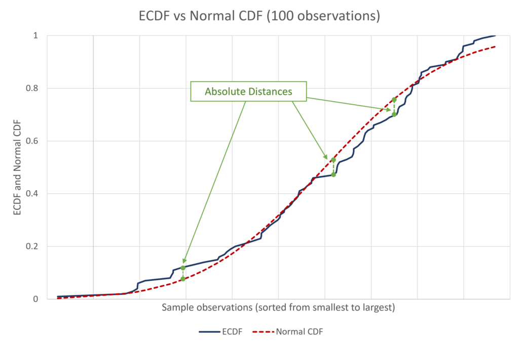
The above graph shows an example of a sample with 100 observations and its comparison with normal distribution. The absolute distances are the differences between the theoretical CDF of normal distribution and the ECDF of the sample (100 observations). The D statistic will be equal to the maximum absolute difference between the two distributions above.
Compare with critical value or obtain P-value
The D statistic obtained in such a way can be compared to the critical value from the tables. Alternatively, there are ways to calculate the p-value for the statistic as well. Statistical software packages make this easy by estimating everything for us.
If the D statistic is greater than the critical value or the p-value is less than 0.05, we reject the null hypothesis. In such a case, we can conclude that the sample does not follow the theoretical distribution. Alternatively, if the D statistic is less than the critical value or the p-value is greater than 0.05, we can conclude that the sample belongs to the theoretical distribution.
In our example of the sample with 100 observations, the results of the Kolmogorov Smirnov test were as follows:
| Kolmogorov Smirnov test: One sample (Normal distribution) | D | P-value |
| 0.0784 | 0.521 |
According to these results, we can conclude that the sample is normally distributed. This is because we cannot reject the null hypothesis that the sample follows the theoretical distribution (normal distribution in this example).
Two sample Kolmogorov Smirnov test
Statement of the hypothesis
The Two sample KS test is used to compare the distributions of two different samples or data. This test shows whether the two samples come from the same distribution or not. The null and alternate hypothesis for the two sample test can be stated as follows:
H0: the two samples come from the same distribution
HA: the distributions of the two samples are statistically different
Calculate the ECDF of the samples
In the one sample KS test, we calculated the ECDF of the sample and compared it with theoretical CDF. However, we have to estimate the ECDFs of both samples in the Two sample KS test. Then, we have to compare the two ECDFs to decide whether the samples belong to the same distribution or not.
The formula for estimating the ECDF stays the same as before:

We can obtain the ECDF of both samples by applying this formula to each sample separately. Let us consider a small example for illustration purposes:
| Sample A (Ordered from smallest to largest) | Ranks | ECDF = pi/n | Sample B (ordered from smallest to largest) | Ranks | ECDF |
| 33 | 1 | 1/10 = 0.1 | 35 | 1 | 0.1 |
| 35 | 2 | 2/10 = 0.2 | 36 | 2 | 0.2 |
| 36 | 3 | 0.3 | 38 | 3 | 0.3 |
| 37 | 4 | 0.4 | 39 | 4 | 0.4 |
| 38 | 5 | 0.5 | 41 | 5 | 0.5 |
| 42 | 6 | 0.6 | 44 | 6 | 0.6 |
| 43 | 7 | 0.7 | 45 | 7 | 0.7 |
| 44 | 8 | 0.8 | 47 | 8 | 0.8 |
| 46 | 9 | 0.9 | 48 | 9 | 0.9 |
| 47 | 10 | 1 | 49 | 10 | 1 |
The ECDFs look the same but their distributions will be different because the values or observations in the samples are different.
Calculate the D statistic
The D statistic is similar to that of the One sample test. The difference is in the fact that the comparison is between the distributions of two samples, instead of a theoretical CDF. The formula for the D statistic looks similar as well:

In this case, the D statistic is the maximum absolute difference between the distributions of the two samples. Hence, the logic behind the test and the D statistic remains the same. The difference lies between the use of theoretical CDF in One sample test and ECDF of the second sample in the Two sample test. The visualisation of the distributions in the Two sample test can be accomplished in the same manner:
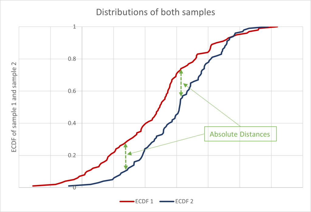
As before, the D statistic will be the maximum absolute difference between the two distributions. Since these ECDFs range from 0 to 1, the D statistic will also range between 0 and 1. The closer the D statistic is to 0, the closer the two distributions are and vice versa.
Compare with critical value or obtain P-value
The interpretation of the results stays the same as before. We reject the null hypothesis if the D statistic is greater than the critical value from the tables. Alternatively, if the p-value is less than 0.05, we can reject the null hypothesis.
Statistical software packages make this step easier because they provide the p-values by default. Let us look at an example of 2 samples with 100 observations each. These are the same samples we used to graph the distributions:
| Kolmogorov Smirnov test: Two samples (100 observations each) | D | P-value |
| 0.27 | 0.001 |
The results of the test make it clear that the two samples come from different distributions. We reject the null hypothesis because the p-value is less than 0.05.
Advantages and limitations of the Kolmogorov Smirnov test
Advantages
- Nonparametric nature: the KS test does not make any assumptions about the distribution of the data. As a result, it can be applied to various types of distributions. This is true in the case of both One sample and Two sample Kolmogorov Smirnov test.
- Different Sample sizes: the test can be applied to data with different numbers of observations. Therefore, different sample sizes are not an obstruction in the application of the KS test.
- Fields of application: the KS test is useful not just in Economics, but in several fields. It is often used in other social sciences, biological sciences, engineering etc.
- Differences in location and shape: when comparing the distributions, the KS test is sensitive to the location as well as the scale of distributions. This implies that it can detect differences in mean, median, standard deviation, skewness, kurtosis and other features of the distributions.
Limitations
- Small sample size: the KS test can be very sensitive to small sample sizes. In small samples, there is a risk of rejecting the null hypothesis even in cases where the distributions are similar.
- Outliers: if the data consists of outlying observations, it can distort the distributions and henceforth the results of the KS test.
- Assumption of independent observations: the test assumes that the observations of the samples are independent of each other. In case of dependence between the observations, the results of the KS test may be invalid.
- Discrete data: the KS test discussed above is applicable only to continuous data and cannot be applied to discrete data. There are certain modifications of the Kolmogorov Smirnov test that can be used for discrete data, but they have their own limitations and disadvantages.
Econometrics Tutorials with Certificates

This website contains affiliate links. When you make a purchase through these links, we may earn a commission at no additional cost to you.