Weighted Least Squares Estimation

The Weighted Least Squares (WLS) method is a special form of Generalized Least Squares estimation. In this method, the original model is transformed so that the variance of residuals becomes constant. Hence, the problem of heteroscedasticity is removed by transforming the variables in the model.

For a meaningful transformation, it is necessary to understand the type or pattern of heteroscedasticity. That is shown by the relationship between the variance of residuals and variables in the model. Based on that relationship, we can decide the weights and transform the original model by implementing those weights on all the variables.

Transforming the original model

Let us consider the following model:

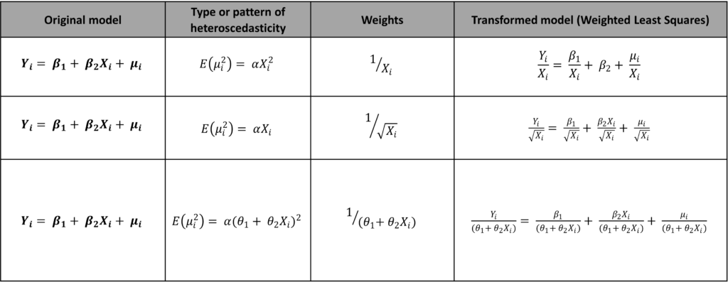
Y_i = β₁ + β₂X_i + μ_i

Suppose, we detect the presence of heteroscedasticity in the above model and the pattern of heteroscedasticity is as follows:

Here, the expected value of squared residuals is a positive function of the independent variable. In other words, with an increase in the value of the squared independent variable, the value of the squared residual also increases. Hence, the variance of residuals will not be constant. But, it will increase with an increase in the value of the independent variable.

In such a case, the original model can be transformed as follows:

Proof of Constant Variance in Weighted Least Squares Transformation

In the transformed model above, we divide all the variables by X_i. The variance of residuals in this transformed model is constant, which can be proved as follows:

We already know that α is a constant, thus, the expected value of transformed squared residuals is constant. Hence, the variance of residuals becomes constant (α) after transforming the original model. In this example, the weights in Weighted Least Squares model are equal to 1/X_i which we used to transform the original model.

The formula for deciding the weights for WLS is simple. The Weights should be equal to the square root of the variables defining the relationship with the expected value of squared residuals. To elaborate, let us consider some examples of different models and types of heteroscedasticity:

Determining the pattern of heteroscedasticity

To implement the Weighted Least Squares, it is necessary to understand the type or pattern of heteroscedasticity because the weights are decided based on its pattern. However, it is usually impossible to know the heteroscedasticity pattern beforehand. Therefore, we will discuss how to discover the underlying pattern of heteroscedasticity.

Glejser’s test of heteroscedasticity can help determine the form of heteroscedasticity. In this, the absolute values of the error term are regressed on the independent variables of the model using different functional forms.

Step 1

Estimate the original OLS model and obtain the residuals. Let us consider the same model as before:

Y_i = β₁ + β₂X_i + μ_i

We can easily obtain the residuals after estimating the model.

Step 2

Perform OLS estimation with |μ_i| (absolute value of μ_i) as the dependent variable and independent variables from the original model (X_i, in this example). Use different functional forms to represent different types of patterns. Some examples of these patterns can be:

Many other functional forms can be tried to determine the pattern. The function that gives the best statistically significant results from the OLS estimation of these equations, represents the pattern or type of heteroscedasticity. As mentioned earlier, that pattern can be used to define the weights for Weighted Least Squares.

The disadvantages of Weighted Least squares

Interpretation Difficulties: the WLS can make the interpretation of coefficients extremely challenging. It changes the variables in the model by transforming them. Since the variables are not in their original form, the interpretation becomes complex. The weights assigned to the variables must be kept in mind while interpreting the results.
Choosing the weights: the choice of weights is usually made with the help of some assumptions related to the pattern of heteroscedasticity. There is a huge possibility of making an error in the choice of weights. The results from the model can be affected by these choices and assumptions.
Possibility of biased results: it is possible that the choice of weights or the assumptions about the pattern of heteroscedasticity is flawed. This can cause the estimates to be biased. Moreover, it can lead to entirely incorrect predictions and conclusions from the model.
Effect of outliers: the results of WLS can be sensitive to outliers and interfere with the results. This happens because the weights can end up having a disproportionate effect on the outliers.
The problem of Overfitting: in the method defined above, the weights are decided based on Glejser’s test and several functional forms. However, this procedure is conducted on the same data that is used to estimate the WLS model. This can result in overfitting and causing the model to perform well for the given data but poorly for any out-of-sample predictions.