Heteroscedasticity is a situation where the variance of residuals is non-constant. Hence, it violates one of the assumptions of Ordinary Least Squares (OLS) which states that the residuals are homoscedastic (constant variance). In heteroscedasticity, the residuals or error terms are dependent on one or more of the independent variables in the model. Therefore, their values are correlated with the values of those independent variables. For instance, if an increase in the value of the independent variable leads to an increase in the value of residuals. This will lead to increased variance of residuals with an increase in the independent variable. In general, any kind of relationship between residuals and independent variables can also lead to heteroscedasticity.
Econometrics Tutorials with Certificates

Causes of heteroscedasticity
Some of the most common causes of heteroscedasticity are:
- Outliers: outliers are specific values within a sample that are extremely different (very large or small) from other values. Outliers can also alter the results of regression models and cause heteroscedasticity. That is, outlying observations can often lead to a non-constant variance of residuals.
- Mis-specification of the model: incorrect specification can further lead to heteroscedastic residuals. For example, if an important variable is excluded from the model, its effects get captured in the error terms. In such a case, the residuals might exhibit non-constant variance because they end up accounting for the omitted variable.
- Wrong Functional form: Misspecification of the model’s functional form can cause heteroscedasticity. Suppose, the actual relationship between the variables is non-linear in nature. If we estimate a linear model for such variables, we might observe its effects in the residuals in the form of heteroscedasticity.
- Error-learning: let us consider an example for this case. Errors in human behaviour become smaller over time with more practice or learning of an activity. In such a case, therefore, errors will tend to decrease. For example, with the skill development of labour, their error will decrease leading to lower defective products in the manufacturing process or a rise in their productivity. Hence, error variance will decrease in such a setup.
- Nature of variables: for instance, an increase in income is accompanied by an increase in choices to spend that extra income. This further leads to discretionary expenditure. In such a case, error variance will increase with an increase in income. A model with consumption as a dependent variable and income as an independent variable can have an increasing error variance. Hence, the nature of variables and their relationships can play a huge role in this phenomenon.
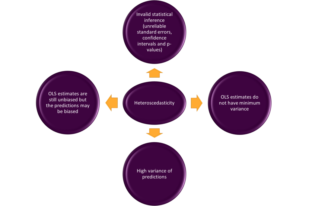
Consequences of heteroscedasticity
The major consequences of heteroscedasticity can be summarized as follows:
- Validity of statistical inference: standard errors, confidence intervals, p-values and other tests of significance are no longer reliable in the presence of heteroscedasticity. This is because OLS standard errors assume constant variance of residuals. The tests of significance are based on these standard errors. In heteroscedasticity, error variance is non-constant, therefore, OLS standard errors are not applicable. As a result, it is not advisable to rely on confidence intervals and p-values.
- The variance of estimates: OLS estimates no longer have minimum variance property because the variance of residuals is not constant. The coefficients end up having larger standard errors and lower precision in the presence of heteroscedasticity. Hence, OLS estimators become inefficient in the presence of heteroscedasticity.
- Predictions: the forecasted or predicted values of the dependent variable based on a heteroscedastic model will have high variance. This is because the OLS estimates are no longer efficient. The variance of residuals is not minimum in presence of heteroscedasticity due to which the variance of predictions is also high.
- Biasedness: the unbiasedness property of OLS estimates does not require a constant variance of residuals. However, the predictions from a heteroscedastic model can still end up being biased, especially in the case of observations with large residuals.
Tests for detecting heteroscedasticity
There are a large number of tests available to test for heteroscedasticity. However, some of those tests are used more often than others. The most important heteroscedasticity tests, their limitations and their uses are as follows:
| Heteroscedasticity test | Limitations | When to use |
| Graphical method | This method involves eyeballing the graphs. The pattern between residuals and independent variable/fitted values may not always be clear. Moreover, it might be affected by the subjective opinions of researchers. | It is generally advised to implement the residual vs fitted plots or residual vs independent variable graphs after every regression. These graphs can provide important insights into the behaviour of residuals and heteroscedasticity. |
| Breusch-Pagan-Godfrey test | It is very sensitive to the assumption of normal distribution of the residuals | This test can be employed if the error term or residuals are normally distributed. Therefore, it is advisable to check the normality of residuals before implementing this test. |
| White’s heteroscedasticity test | It generally requires a large sample because the number of variables including the squared and cross products can be huge, which can restrict degrees of freedom. This is also a test of specification errors. Therefore, test statistic may be significant due to specification error rather than heteroscedasticity. | This test does not depend on the normality of error terms and it does not require choosing ‘c’ or ordering observations. Hence, it is easy to implement. However, it is important to keep the limitations in mind. |
Other important tests
| Heteroscedasticity test | Limitations | When to use |
| Goldfield-Quandt test | ‘c’ or central observations to be omitted must be carefully chosen. A wrong choice may lead to unreliable results. For multiple independent variables, it becomes difficult to know beforehand which variable should be chosen to order the observations. Separate testing is required to determine which variable is appropriate. | This test is preferred over the Park test and Glejser’s test. Goldfeld and Quandt suggested that c=8 and c=16 are usually appropriate for around n=30 and n=60 observations respectively. |
| Park test | The error term within the test itself may be heteroscedastic, leading to unreliable results. | This test can be used as a precursor to the Goldfeld-Quandt test, to determine which variable is appropriate to order observations. |
| Glejser’s Heteroscedasticity test | Similar to the Park test, the error term within the test may be heteroscedastic. | This test has been observed to give satisfactory results in large samples. However, the most important usage of this test is to determine the functional form of heteroscedasticity before implementing Weighted Least Squares (WLS). This test can be used to determine the weights in WLS, depending on the relationship between the variance of residuals and independent variables. |
Solutions to the problem of heteroscedasticity
Several approaches can be adopted to counter heteroscedasticity. Some of these methods are as follows:
Robust Standard Errors
The usual OLS standard errors assume constant variance of residuals and cannot be used in heteroscedasticity. Instead, robust standard errors can be employed in such cases. These allow a non-constant variance of residuals to estimate the standard errors of coefficients. Moreover, the HC3 Robust standard errors have been observed to perform well in heteroscedasticity.
Weighted Least Squares
The Weighted Least Squares technique is a special application of Generalized Least Squares. The variables in the model are transformed by assigning weights in such a manner that the variance of residuals becomes constant. The weights are determined by understanding the underlying relationship or form of heteroscedasticity. Glejser’s heteroscedasticity test can also be used to determine the heteroscedastic relationship between residuals and independent variables.
Transforming the variables
Transforming the variables can help reduce or even completely eliminate heteroscedasticity. For example, using log transformation reduced the scale of all the variables. As a result, the scale of residual variance also decreases which helps mitigate the problem of heteroscedasticity. In some cases, the problem of heteroscedasticity may be totally eliminated. In addition, log transformation provides its own benefits in economics by letting us study the elasticities of variables.
Non-parametric methods
Non-parametric regression techniques make no assumptions about the relationship between dependent and independent variables. In OLS, the assumption of constant residual variance is violated by heteroscedasticity. However, there are no assumptions to violate in the case of non-parametric methods. Estimation techniques such as Kernel regression, Splines and Random Forest fall under the category of non-parametric methods. These provide a lot more flexibility in estimating complex relationships.
Related Posts
Econometrics Tutorials with Certificates

This website contains affiliate links. When you make a purchase through these links, we may earn a commission at no additional cost to you.
Best source
Thank you!!!