The Production Possibility Curve is also referred to as the product transformation curve and production possibility frontier. Firms often produce more than one outputs that are closely related to each other. The production possibility curve (PPC) shows various combinations of two products that can be produced by a firm with the given level of inputs (labour and capital).
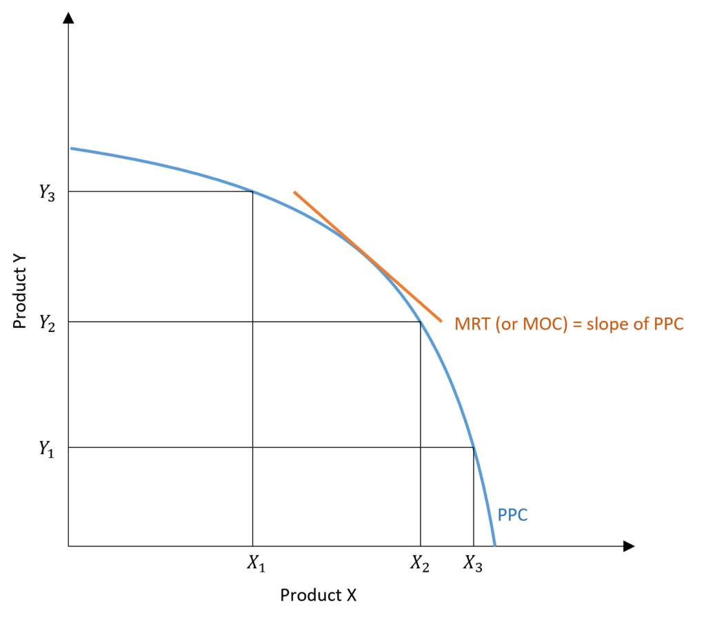
The PPC in the diagram shows all the combinations of products X and Y that can be produced by a firm with the given level of labour and capital. The PPC is a downward sloping curve because there is a trade-off between the two products. To produce more of one product, the firm has to forego some quantity of the other product. This is because the level of inputs remains the same. For instance, to produce more of product X, the firm has to divert its inputs from Y to the production of X and has to reduce the production of Y.
This website contains affiliate links. When you make a purchase through these links, we may earn a commission at no additional cost to you.
Econometrics Tutorials


slope of PPC: marginal rate of transformation (MRT)
The slope of the PPC shows this trade-off. That is, some quantity of one good has to be foregone to produce an extra unit of the other product, with inputs that are given. It is also known as the Marginal Rate of Transformation (MRT) and Marginal Opportunity Cost (MOC) and can be expressed as:

The price is determined by the marginal costs of products under perfect competition. This implies that the price ratios of two goods are equal to the ratio of their marginal costs.
The output mix or the change in output (dY/dX) will be equal to the ratio of prices (and the ratio of marginal costs) of both goods. Therefore, every point on the production possibility curve shows a different price ratio of goods (MRT/MOC/ slope).
economies of scope
The shape of PPC and its slope (MRT) shows the existence of economies of scope. The PPC is concave to the origin and the MRT increases as we move along the PPC. The joint production of products X and Y has some cost benefits. These are known as the Economies of Scope which allows the firm to produce more of both products with joint production from given inputs. If these products were produced by different firms, then the output of both X and Y would be less because there will be no economies of scope.
To illustrate with an example, some products like chicken and eggs can be produced together for additional benefits. Poultry farms produce both eggs and chicken as products. They can benefit from joint production to earn economies of scope because both require the same inputs. It is better to produce both, than to produce only chicken or only eggs.
If PPC was a straight line, then, it means that the firm does not experience economies of scope. There will be no difference in the output of X and Y, irrespective of joint production or producing them separately. The economies of scope can result from sharing of the same inputs, joint marketing or management. In certain cases, the production of one output automatically produces the other as a by-product, as is the case of chicken and eggs.
Measuring Economies of Scope
Sometimes, the joint output is greater than producing both outputs separately in separate firms. Economies of scope can be measured through the cost of the firm. With economies of scope, a firm can produce more output from joint production with the same level of inputs, as compared to two independent firms producing X and Y separately. Hence, it will cost a single firm less to produce a given output as compared to two firms. The degree by which the costs are lesser can be used to measure economies of scope.
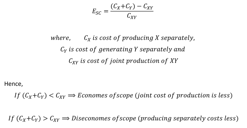
Finally, diseconomies of scope would simply mean that the production of X and Y is interfering with each other. That is, it is costing more to produce both goods together.
Important: economies of scope and economies of scale are not directly related. A firm can experience economies of scope along with diseconomies of scale. Or, a firm may have no economies of scope with economies of scale.
Econometrics Tutorials