The Bernoulli distribution stands as the cornerstone of discrete probability distributions. It serves as a bedrock for various statistical and econometric paradigms, enabling the probability calculation for dichotomous outcomes – these range from decisive victories and failures to simple yes-no decisions. Mastery of the Bernoulli distribution is essential for professionals in economics, finance, or the analytics field.
Essentially, the Bernoulli distribution represents a single experiment involving two alternatives: success, usually indicated by 1, and failure, by 0. A crucial parameter, p, signifies the probability of success, holding values between 0 and 1. This distribution acts as a precursor to more intricate models, like the binomial, prevalently applied in economics and econometrics settings.
Econometrics Tutorials with Certificates

What is Bernoulli Distribution?
The Bernoulli distribution serves as a foundational framework for probability calculations. It is used in scenarios presenting only two possible outcomes, known as binary situations. For example, in processes like passing or failing, winning or losing, or deciding yes or no. Hence, we can think of it as a mathematical mirroring of a coin toss. The probability of attaining success is denoted by ‘p,’ while the probability of failure is calculated as “1 – p“. This distribution stands as a foundational aspect of the broader binomial distribution. It becomes particularly relevant in contexts requiring only a single experimental trial to ascertain success or failure.
Binary Outcomes and Constant Probability
Jacob Bernoulli, a noteworthy Swiss mathematician, lends his name to the Bernoulli distribution. It finds application in discrete probability settings, where the variable under consideration assumes the value 1 with the probability “p” and 0 with the probability “q” or “1 – p“.
Therefore, within the Bernoulli framework, scenarios are constrained to two outcomes, denoted as success (1) or failure (0). Notably, the likelihood of success, represented by ‘p,’ maintains a constant value throughout Bernoulli’s trials.
Furthermore, the Bernoulli distribution is not isolated in its utility. Rather, it acts as a cornerstone for various other discrete distributions. Some of these include the binomial distribution, geometric distribution, and negative binomial distribution. As part of the categorical distribution cluster, it is recognized as a distinctive form within the field of statistical distributions.
Probability Mass Function of Bernoulli Distribution
As discussed, a variable solely adopts one of two states: success (designated as 1) or failure (etched as 0). Its application is also prevalent in disciplines such as economics, finance, and business, offering insights into events pivoted on dual outcomes.
The probability mass function underpinning the Bernoulli realm assumes the form:

- X signifies the random variable, constrained to 0 or 1.
- “p” denotes the success probability (linked to X = 1).
- Conversely, “1-p” symbolizes the likelihood of failure with X taking the null value.
To succinctly encapsulate, the functional schema emerges thus:
- P(X=0) embodies the prospect of non-success, thus equated to 1-p.
- P(X=1) encapsulates the area of success, appraised simply as p.
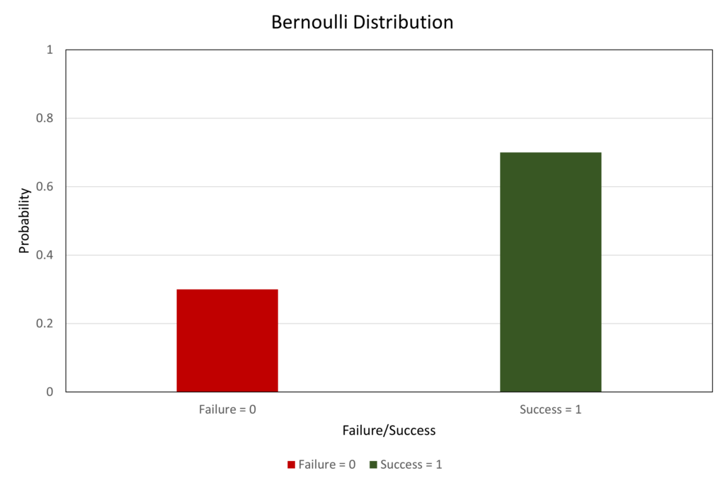
The figure above depicts the probability mass function of the Bernoulli Random Variable with “p = 0.7“. Therefore, the probability of success (1) is 0.7. As a result, the probability of failure (0) is “1 – p = 0.3“.
Mean and Variance of Bernoulli Distribution
The Bernoulli distribution plays a foundational role in statistics, finding broad use in fields such as economics, quality control, and market research. It encapsulates the result of a solo binary event, envisioning the outcome as either “success” or “failure” with exceptional ease.

The expected value, or mean, of a Bernoulli random variable X equates to the likelihood of success or “p”. This also signifies the typical outcome from a trial. For instance, in a group where 75% favour peanut butter, the mean for this preference variable is 0.75.
Calculating the variance for X follows a simple formula: p(1 – p), leveraging “p” as the chance for success. The standard deviation is the square root of variance and is denoted by “√(p(1-p))“. It outlines the expected fluctuation from the mean, unveiling the experiment’s inherent variability and uncertainty.
Hence, a Bernoulli distribution’s mean and variance are directly tied to the probability of success “p“. These characteristics are also indispensable for dissecting and evaluating binary events and their probabilities.
Properties of Bernoulli Distribution
Binary Outcome: The Bernoulli distribution is defined by its unique characteristics. It is a discrete model, limiting outcomes to success (1) or failure (0). This feature also sets it apart, making it ideal for scenarios with binary results.
Fixed Probability: A key attribute is the fixed success probability (p) across all tests. Here, each trial maintains the same success chance, for example, flipping a fair coin will have a 0.5 probability of heads in each toss. Moreover, the events are self-contained, ensuring one’s result doesn’t alter another’s. For instance, the result (heads or tails) of a coin toss will not affect the result of subsequent coin tosses.
Probability sums to 1: This distribution also guarantees the sum of success and failure odds equals 1. This condition further outlines the completeness and incompatibility of the two outcomes. It’s also an essential principle in probability theory. Therefore, the probability of success and the probability of failure will always sum to 1.
Mean and Variance: For statistical assessments, the expected value of the Bernoulli variable directly equates to its success likelihood, E(X) = p. Meanwhile, its variance is the product of “p” and its complement, Var(X) = p(1-p). These calculations underline its utility across disciplines like quality assurance and finance, aiding in critical decision-making.
Moreover, the Bernoulli distribution lays the foundation for more intricate models like the Binomial distribution. Through this progression, it’s possible to analyze the collective success in a sequence of independent trials. This power is also vital in statistical investigations, enabling predictive analytics and sophisticated strategic planning.
Bernoulli Trials
The Bernoulli distribution, crucial in probability theory, serves as a model for experiments yielding two outcomes: success and failure. Here, a Bernoulli trial encapsulates a single observation conforming to this distribution, denoted by a binary variable, either 1 (for success) or 0 (for failure). Moreover, such trials are unequivocally independent. The outcome of one trial is inert towards any other, with fixed success (p) and failure (q) probabilities across all trials.
Conditions of Bernoulli Trials
Hence, the essential tenets of Bernoulli trials include:
- Fixed and finite number of trials
- Independent trials; the outcome of any one trial has no sway on others
- Thus, there exist only two outcomes, success or failure, with steady probabilities
Illustrations of Bernoulli trials range from tossing a coin to pressing a light switch. Each feat materializes into a singular, binary result, like head or tail, and is underpinned by unchanging success (p) and failure (q) odds.
The Bernoulli distribution acts as the single-trial case within Binomial models. It forms the cornerstone for comprehending more elaborate probabilistic structures, including the Binomial and Multinomial distributions.
Examples of Bernoulli Distribution
The Bernoulli distribution applies to scenarios featuring two outcomes only: successful or failed events. As a result, it serves a myriad of applications in both simple daily events and complex mathematical analyses. We will examine several examples that highlight the breadth of scenarios matched by this distribution.
A classic demonstration comes from tossing a fair coin. The likelihood of obtaining a head, considered a success, equals 0.5, mirroring the 0.5 chance of obtaining a tail, a failure. These coin flips map perfectly onto the framework of Bernoulli distribution, using a single random variable to encode the outcome of each flip.
Considering a student’s likelihood of passing a test opens another avenue for Bernoulli’s utility. It marks passing the exam as success and failing as the opposite outcome.
Another example to consider is the probability of default on a loan. Financial institutions can employ Bernoulli distribution in such a situation to predict the probability of default on loans. An individual taking a loan can be considered a Bernoulli trial, who faces two outcomes: default on the loan or pay it back.
These applications showcase the Bernoulli distribution’s proficiency in scenarios where outcomes are binary and success odds remain consistent across multiple trials. Therefore, its widespread adoption spans areas like drug testing, consumer analytics, financial market modelling, ensuring product quality, and computer simulations of various kinds.
Applications in Economics and Business
Quality Control
In manufacturing, the Bernoulli model is also pivotal for product quality assessment. It aids in calculating the chance that an item adheres to predefined quality metrics. Hence, this approach enables firms to gauge the overall quality of their outputs and strategize enhancements. Furthermore, such analyses are critical in maintaining consistent product excellence.
Market Research
Within market research, the Bernoulli distribution shines, particularly for queries eliciting yes/no responses. Consider customer satisfaction surveys, where results are categorized as “satisfied” or “dissatisfied”. Through such categorization, companies can glean profound insights into client preferences. This, therefore, informs data-based strategies aimed at product and service improvement for superior customer satisfaction.
Risk Assessment
Bernoulli distribution also finds application in risk modelling, especially for events with binary outcomes like defaults. Understanding these event probabilities is vital for ensuring sound risk management across sectors. Armed with insights into the probability of such events, organizations and financial entities can devise better risk mitigation strategies.
In summary, the Bernoulli distribution is instrumental in leveraging binary outcomes for critical business decisions. Hence, by simplifying the analysis of constant probability events, it becomes an indispensable asset in the business analytics toolkit. Its adaptability and accuracy in modelling binary scenarios serve various industries and applications effectively.
Use of Bernoulli Distribution in Econometrics
In the realm of econometrics, the Bernoulli distribution plays a pivotal role, more specifically within the likelihood functions of logit and probit models. These sophisticated tools are crucial for assessing binary dependent variables. Such variables might include a consumer’s decision to purchase or not, or a chance to default on a loan. At their core, the likelihood functions in these models pivot around the Bernoulli distribution. This choice is not incidental; it accurately captures the probability of binary outcomes.
Likelihood Functions of Logit and Probit Models
The logit model, predicated on a logistic function, encapsulates the binary essence of the dependent variable. In contrast, the probit model leverages a normal cumulative distribution function. Yet, despite their differences, both models root their likelihood calculations in the Bernoulli distribution. Hence, this foundation is instrumental in gauging the likelihood of the observed results.
For the logit model, its likelihood function intricately intertwines with the Bernoulli distribution. Here, modelling the probability of success involves a logistic function. Conversely, the probit model takes a different path. It employs the normal cumulative distribution function to estimate the probability of a binary outcome.
The strategic application of the Bernoulli distribution underpins research into what affects the likelihood of binary outcomes. This approach is rich in its potential to inform decision-making and shape policy by providing in-depth insights.
With the integration of the Bernoulli distribution into models such as logit and probit, skilled econometricians can model binary outcome probabilities with finesse. Hence, these methodologies are of paramount importance in various fields, including business, finance, and policy studies.
Bernoulli Distribution vs Binomial Distribution
The Bernoulli distribution and Binomial distribution share a common thread but diverge significantly in their functionality and breadth of application. A Bernoulli distribution is suited for scenarios where we witness but one instance with two likely results, as in the case of a coin toss, where the outcome is either heads or tails. In contrast, the Binomial model sees the light in multiple, independent trials of the said single event (coin toss), that is, the number of successes (heads or tails) in multiple coin tosses.
The crux of the disparity between these distributions lies within their unit of analysis. The Bernoulli distribution thrives in scenarios with binary outcomes, effectively encapsulating triumph (1) or defeat (0). Conversely, the Binomial distribution extends from the Bernoulli, accommodating multiple ‘successes’ amidst a specified number of trials.
Therefore, this divergence culminates in the crafting of individual formulas and the delineation of precise applications. While the Bernoulli encompasses a singular parameter, the success probability “p”, the Binomial broadens the horizon with a duo of parameters, the number of trials denoted as “n” and probability of success as “p”.
| Characteristic | Bernoulli Distribution | Binomial Distribution |
| Number of Trials | Single trial | Multiple trials |
| Outcomes | Binary (Success or Failure) | Number of successes in multiple trials |
| Parameters | p (probability of success) | n (number of trials), p (probability of success) |
| Expected Value | E(X) = p | E(X) = n * p |
| Variance | Var(X) = p (1-p) | Var(X) = n * p * (1-p) |
Moreover, the Bernoulli distribution is a special case of Binomial distribution when the number of trials equates to 1. It’s therefore viewed as a more elemental, yet no less crucial, facet of the Binomial distribution.
Conclusion
The Bernoulli distribution is a core probability model. It explores the chance of success or failure in a single attempt or experiment. Furthermore, its utility spans fields like economics, business statistics, and econometrics. Here, it aids in analyzing binary results and guiding decisions.
The Bernoulli distribution, despite its known constraints, is a vital concept in statistics. It thrives on the assumptions of fixed probabilities and independent and binary outcomes. Though these conditions may not always mirror the real world, its straightforwardness and adaptability position it as a foundational element for many analyses. The process of Bernoulli trials – where trials are independent with a constant success probability – lays the groundwork for the binomial distribution and other more intricate models.
To recap, the Bernoulli distribution proves invaluable for working with binary events. It is pertinent in varied contexts such as clinical trials, quality assurance, market studies, and hazard evaluation.
Econometrics Tutorials with Certificates

This website contains affiliate links. When you make a purchase through these links, we may earn a commission at no additional cost to you.