The binomial distribution stands as a cornerstone in statistical theory. It depicts the probability of achieving a certain number of successes or failures over multiple Bernoulli trials. Hence, its primary application lies within scenarios embodying two outcomes, specifically success and failure, over several trials. A classic example is the number of heads or tails in multiple coin tosses, with success represented by heads (50% chance) and failure by tails (50%).
Another example we can consider is that of predicting student behaviour. For instance, given that around 70% of students submit their statistics homework on time, one could use the binomial model to calculate the likelihood of at least 40 timely submissions in a class of 50.
Binomial distribution finds application in numerous settings, from manufacturing quality control to gauging customer satisfaction and even appraising marketing initiatives. This is due to its design for scenarios featuring fixed, independent trials, each characterized by the same set probability of outcomes.
Econometrics Tutorials with Certificates

Basic Principles of Binomial Distribution
To effectively apply binomial distribution across disciplines, it’s also critical to master its core principles. Furthermore, this model hinges on two discrete trial outcomes, success and failure, which reflect the essence of Bernoulli trials. Every trial is characterized by the unchanging chance of success and the independence of trials from each other.
Mean and Variance
The binomial distribution is designated as:
X ~ B(n, p)
It involves a fixed number of trials (n) and a success probability (p) constant in each. For example, investigating 100 individuals with a specific gene where disease contraction has a 0.70 chance, resulting in a B(100,0.7) distribution. Moreover, the mean and variance are crucial metrics of the binomial distribution:

Assumptions and Criteria
Furthermore, for binomial distribution application, several assumptions and criteria must be adhered to:
- The number of trials (n) is unchanging.
- Independence characterizes these trials.
- Success or failure marks the end of each trial.
- The likelihood of success (p) remains uniform across all attempts.
These prerequisites bolster the reliability of predicted outcomes, allowing for direct or software-aided precise probability calculations.
The binomial distribution and its application is critical in economic projections and scenarios with essential binary or discrete probability aspects.
Probability Mass Function of Binomial Distribution
In the realm of probability theory, the probability mass function (PMF) illuminates the discrete random variable’s probability distribution. Hence, the binomial distribution determines the likelihood of a precise number of successes (k) during a predetermined series of trials (n). Its application in economic statistical analysis is also pivotal, driving insightful forecasts.

Moreover, the PMF’s core tenets dictate that probability p(X) remains nonnegative for all feasible “x” and its summation across all likely values equates to 1. These characteristics also underpin the PMF as a thorough probability model for random experiments. It is instrumental alongside the cumulative distribution function (CDF) in evaluating the probabilities of events and the number of successes.
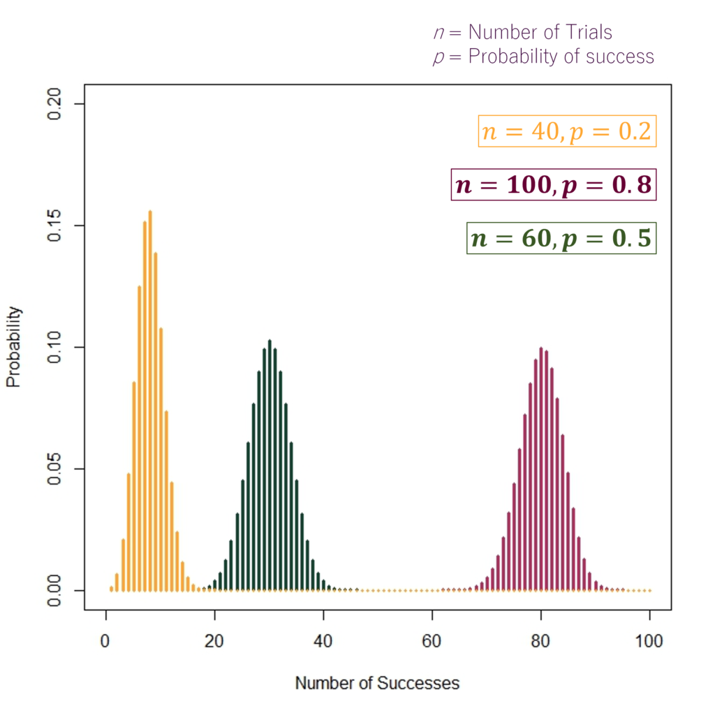
Probability Mass Function: Examples
Cumulative Distribution Function: Examples
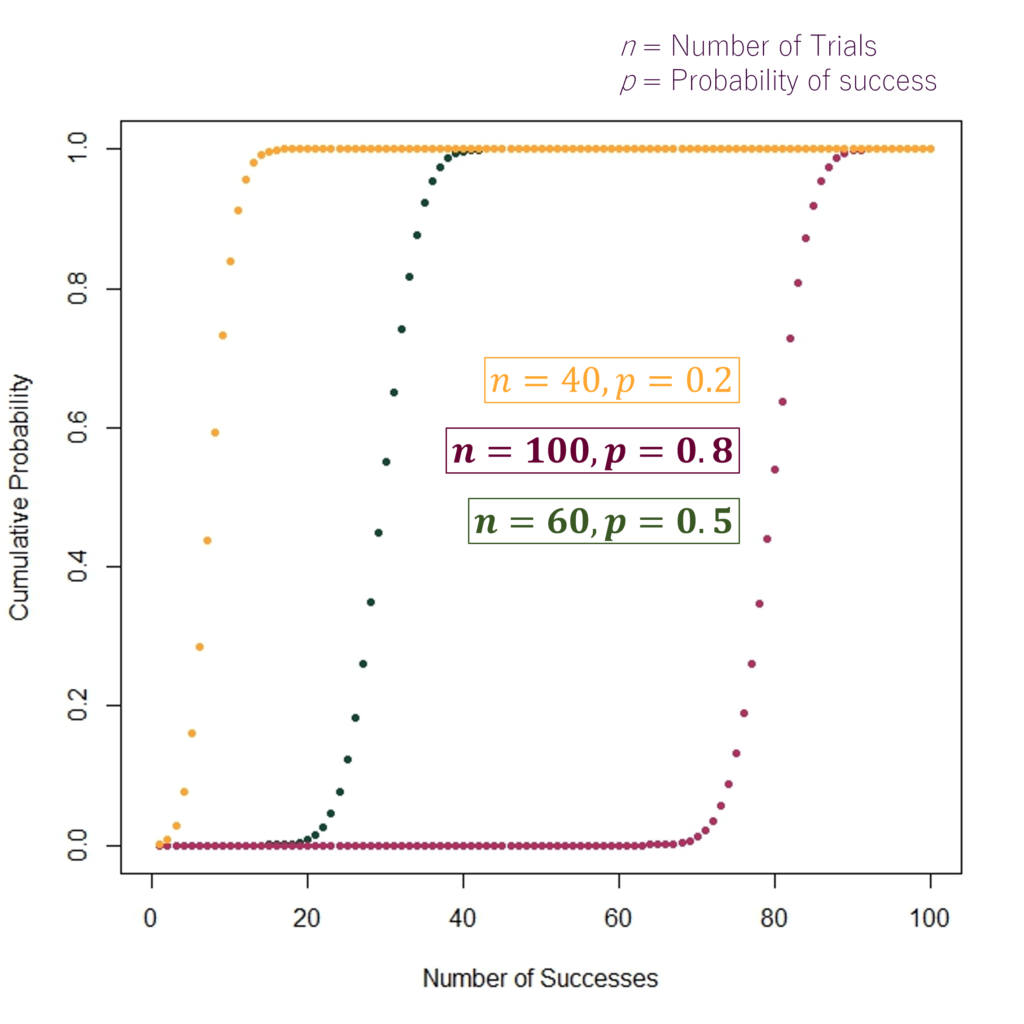
Some examples of Probability Mass Functions and their corresponding CDFs are shown in the diagrams above. Hence, the different number of trials (n) and probability of success (p) give us vastly different distribution functions. For instance, the first PMF and CDF in orange have 40 trials and 0.2 probability of success.
Similarly, the middle PMF and CDF in dark green are based on the number of trials (n) = 60 and probability of success (p) = 0.5. We can also get a good idea about the probability of “k” number of successes just by looking at the graphs. Let us consider the example of the PMF shown in the middle (“dark green”) with n = 60 and p = 0.5. The probability of X = k = 30 or exactly 30 successes out of 60 trials looks to be a little over 0.10 (the exact probability comes out to be 0.10258).
Binomial Distribution Examples
The exploration of binomial distribution’s application spans a wide range, including economics. Calculating the likelihood of attaining specific success numbers aids in activities such as maintaining quality standards, assessing the efficiency of policies, and predicting economic shifts. This model inherently features a set number of trials with outcomes that are binary, either succeeding or failing, also based on a given success probability per trial. A common application can be seen in evaluating the defect tally of a product batch. As a result, it enables firms to anticipate and uphold production criteria.
More broadly, the binomial probability distribution’s essence lies in its governing parameters: independent trial counts and success likelihood. A notable case is also found in a health examination with a certain success rate across trials. Here, the mean and variance values highlight the distribution’s key aspects, essential for making valid predictions about the effectiveness of medicines or medical procedures. Therefore, understanding these metrics is pivotal in applying the model effectively.
Examining binary economic events, like trade decisions in the stock market, further showcases the usefulness of the distribution. The mean value calculation over trades informs the success chances in trades. This approach can, therefore, be instrumental in crafting profitable trading strategies.
The binomial distribution plays a foundational role in the realm of probability theory and its uses are also plentiful. It assists in gauging new policy impacts, risk analysis in financial activities, and maintaining quality assurance.
Bernoulli Distribution and Binomial Distribution
The Bernoulli distribution characterizes a variable with two outcomes, often identified as success and failure or numerically as 1 and 0. For instance, consider a coin toss where heads represents success and the coin has a 50% chance of landing that way. When numerous independent trials of such a process occur, we refer to it as a Binomial distribution. An example is the case of four coin flips, aiming to count the number of head outcomes, under the same 50% probability assumption, denoted by “p“, and conducted four times, denoted by “n“.
Binary variables, like passing or failing an exam, are well-modelled within this framework. Assuming a 95% passing chance also implies a 5% possibility of failure. This context also fits the criteria of a Bernoulli process, featuring one trial with two distinct results. Conversely, when aiming to derive the likelihood of passing five exams out of five, the binomial distribution’s utility becomes evident, yielding a probability of approximately 0.774 or about 77.4% chance of passing 5 out of 5 exams. Such an example further illustrates the assembly of binomial scenarios through multiple Bernoulli tests.
Defined through “n” and “p“, the binomial distribution portrays the probabilities of the success count out of “n” independent experiments. Hence, its probability mass function computes the chance of accruing exactly “k” successes from “n” trials. While comparing it to the Bernoulli distribution, we have to deal with an extra parameter “n” or the number of trials. Therefore, this extra parameter “n” leads to a modified Probability Mass Function for Binomial Distribution. Moreover, the mean and variance are slightly modified as well:
Bernoulli Distribution

Binomial Distribution
This highlights the binomial distribution’s power, further leveraging the Bernoulli process for succinct statistical computations and estimations.
Role of Binomial Distribution in Economics
Binomial distribution significantly impacts economics, offering a strong probabilistic framework. It’s vital for making predictions in economics and also enhances financial decision-making processes.
Application in Economic Forecasting
Economic forecasting hinges on predicting binary outcomes, like loan default risk. For illustration, a bond portfolio’s chance of default can be predicted using Binomial distribution. As a result, this probability can be crucial for anticipating returns and risks. Moreover, the Binomial CDF also holds a significant use in economics and finance. In a hypothetical scenario, the likelihood of a stock trader making 600 or more successful trades out of 1,000 at a 0.60 success rate is 0.51373. It highlights binomial distribution’s role in precise financial forecasts and strategic choices.
Risk Assessment in Finance
The Binomial distribution is also key in managing binary economic outcomes like investment results. Consider the probabilities within a bond portfolio: one default may have a 24% chance, two defaults at 2.50%, and three defaults may drop to 0.10%. This information empowers investors and analysts to strategize effectively and lower risks. This in turn enhances the accuracy of financial forecasts and facilitates well-informed decisions.
Finance leans heavily on binomial distribution for gauging default risks, and further enriching risk management practices. Take for instance the calculation of the probability that multiple fraudulent credit card charges might occur. Hence, this exercise allows financial entities to mitigate potential fraud threats effectively.
Quality Control and Consumer Satisfaction
The breadth of binomial distribution’s application spans various economic scenarios. This includes detecting defective goods in manufacturing, analyzing drug efficacy in clinical trials, and extracting insights through market research. Its versatility makes it an irreplaceable tool for both economists and financial analysts.
Additionally, estimating the likelihood of product returns is instrumental for firms in controlling inventory and preventing losses. Such risk assessments form the bedrock for devising protective strategies.
Other Applications
For policymakers, predictive analysis through binomial distribution is a boon. It aids in envisaging how economic policies might pan out across various scenarios. One application is linking marketing conversions with policy impacts to gauge each initiative’s success. Moreover, in clinical trials, it helps in analyzing the probability of patient groups encountering side effects, contributing to more informed health policy planning. This approach to modelling economic scenarios strengthens the basis for data-centered policy decisions, fostering the implementation of strategies that are both focused and effective.
Conclusion
The binomial distribution provides a robust foundation for professionals engaged in statistical analysis, risk management, and economic decision-making. Through a deep comprehension of its core tenets, economists enhance their ability to forecast likelihoods across diverse domains, ranging from financial activity to market trends.
In the realm of manufacturing, binomial distribution is instrumental in quality control. It empowers factories to probabilistically assess defective items during inspections. This capability is crucial for maintaining product excellence and optimizing the use of resources. In the field of health sciences, its application facilitates precise forecasts in clinical trials. It supports the process of bringing new pharmaceuticals to market by improving the accuracy of approval forecasts.
Summing up, Binomial distribution is a cornerstone in the architecture of statistics, economic prediction, market scrutiny, risk evaluation, and policy framing. Its capacity to model discrete binary outcomes, with a known probability, over a fixed number of trials, renders it indispensable for precise prognostications and judicious decision-making in various economic spheres. This solidifies its vital place in the realm of statistical analysis and probabilistic forecasting.
Econometrics Tutorials with Certificates

This website contains affiliate links. When you make a purchase through these links, we may earn a commission at no additional cost to you.