Did you know that nearly 99.7% of data points in a normal distribution are within three standard deviations of the mean? This fundamental aspect of the normal distribution, or Gaussian distribution, highlights its significance in statistical analytics and econometric models. Also known for its symmetric bell-shaped curve, this distribution is key for understanding natural occurrences.
The essence of the normal distribution lies in its mean and standard deviation. The mean showcases the data’s central point, whereas the standard deviation reflects how spread out the values are. This setup allows it to closely fit diverse data types, serving as a bedrock for economists, econometricians and data scientists.
Therefore, a grasp of the normal distribution is indispensable for professionals dealing with analytical data or economic studies. It stands as a cornerstone in the realm of statistics and econometrics.
Econometrics Tutorials with Certificates

What is Normal Distribution?
A normal distribution, also known as a Gaussian distribution, encompasses a probability framework symmetric about the mean. This symmetry implies that data points clustering around the mean are more common. Its significance in statistical analysis is underpinned by its frequent occurrence in nature. Moreover, its fundamental properties aid in simplifying the interpretation of complex data sets.
Definition
A normal distribution represents a continuous probability structure for real-valued random variables in the realm of probability theory and statistics. The standard variant, or standard normal distribution, is characterized by a central mean of 0, a variance and a standard deviation of 1. Furthermore, a mere two parameters, namely the mean and standard deviation, succinctly capture the essence of a normal distribution. Moreover, the central limit theorem underscores that the averages of independently and identically distributed variables tend to approximate a normal distribution.
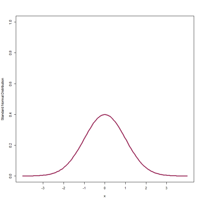
The figure above shows the shape of a Standard Normal Distribution which has a mean 0 and standard deviation of 1.
Properties
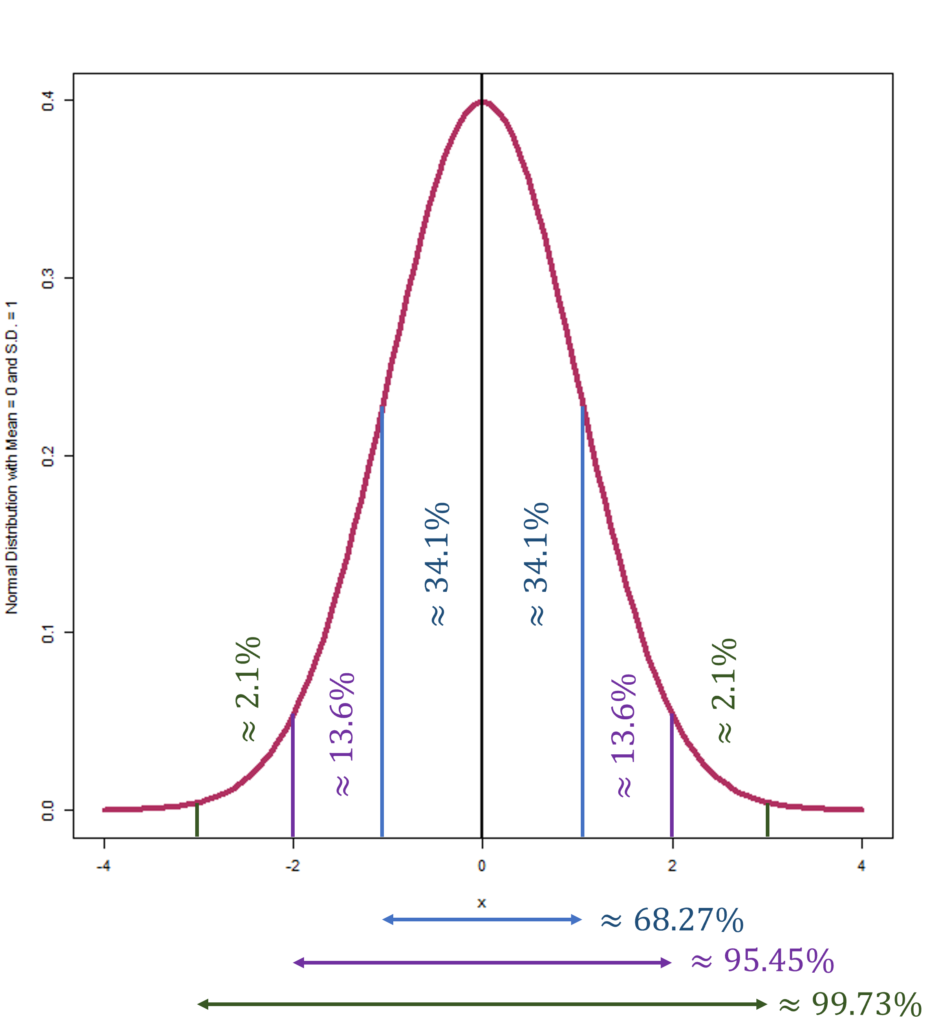
The hallmark of a normal distribution is its symmetry, ensuring zero skewness. It has a kurtosis value of 3.0, depicting a mesokurtic form. Distributions deviating from this value exhibit varying kurtosis characteristics, being either leptokurtic or platykurtic. Such symmetry allows the mean and standard deviation to precisely identify the data’s central tendencies and variabilities. Notably, roughly 68.27% of data fall within one standard deviation, 95.45% within two, and 99.73% within three standard deviations from the mean in normal distribution.
Its application spans diverse arenas, notably in technical financial analysis, owing to its symmetrical and simplistic nature. It also finds wide use in Statistics and Econometric techniques.
Characteristics of Normal Distribution
The normal distribution is defined by its mean and standard deviation. They elucidate the probability distribution along with the center and spread of the data set.
Mean
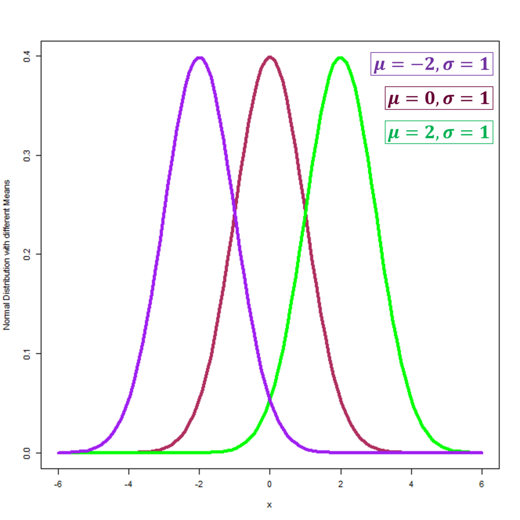
The mean serves as the central spindle of the normal distribution, encapsulating where data concentrates. Therefore, it essentially defines the middle point. Adjusting the mean shifts the curve without altering its symmetry as shown in the figure below. In the context of a standard normal distribution shown in maroon colour with a mean of zero, half of the data points fall below it. This feature is pivotal for assessing central tendencies. The Normal Distributions in the figure have the same standard deviation of 1, but different means of -2, 0 and 2.
Standard Deviation
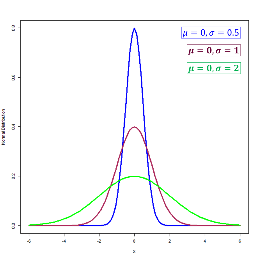
Standard deviation measures how spread out data points are from the mean, thus influencing the curve’s breadth. About 68.27% of the data falls within one standard deviation from the mean, with increasing coverage at further deviations. In the figure below, we can observe 3 different normal distributions which have the same mean of 0. However, their standard deviations are different at 0.5, 1 and 2 which also changes their shape. The Standard Normal Distribution is shown in maroon with a mean of 0 and a standard deviation of 1.
Bell Curve
The bell curve, an iconic graphical depiction, serves to outline the normal distribution’s attributes. This symmetrical plot, with its mean-centered shape, is widely lauded for its capacity to represent statistical data with clarity. Its utility extends across various fields, also aiding in the understanding of data distribution.
Visual Representation
The alignment of the curve’s peak with the mean, median, and mode allows for the division of data into mirror-image sections. By doing so, it simplifies the comprehension of both the spread and central values of a dataset. In the context of the standard normal distribution, specific percentages of data concentrate within defined standard deviations from the mean. In the figures shown above, each normal distribution curve is characterised by mean = median = mode.
Normal Distribution Formula: Probability Density Function
The normal distribution formula or normal probability density function lies at the heart of statistical analysis, serving as a key method for computing probabilities within economic distributions. It is characterized by a probability function utilizing the mean (μ) and standard deviation (σ) to determine the likelihood f(x) of a variable x. Mathematically, this relationship is expressed as:

Furthermore, through z-score standardization, analysts simplify the use of normal distributions. This process mitigates the need for intricate cumulative probability computations, enhancing efficiency.
The versatility of the normal distribution formula also extends to various transformation applications. For example, it facilitates the conversion of any normal distribution into the standard form using Z = (X – μ) / σ. This standardization enables expedited cumulative probability determination for specific value intervals through reference to standardized tables.

Furthermore, the formula’s utility includes approximating the binomial distribution conditionally. Such approximations also simplify otherwise complex statistical analyses, rendering them more accessible and relevant in economic contexts. Mastery of the normal distribution formula empowers economists and financial experts to derive significant insights from raw data. This significantly boosts the accuracy and impact of their analytical and decision-making processes.
Normal Cumulative Distribution Function
The normal cumulative distribution function (Normal CDF) is fundamental in statistical analysis, portraying the likelihood of a normally distributed random variable falling within a specific interval. It is a key element in a myriad of statistical contexts, facilitating extensive analysis.
Definition
The normal cumulative distribution function (CDF) emerges from the integral of the probability density function (PDF) of a normal distribution. Specifically, for the standard normal distribution, Normal CDF or Φ(x) signifies the probability that the standard normal variable Z is less than or equal to a given value of x. This is expressed mathematically by the equation:

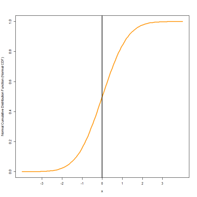
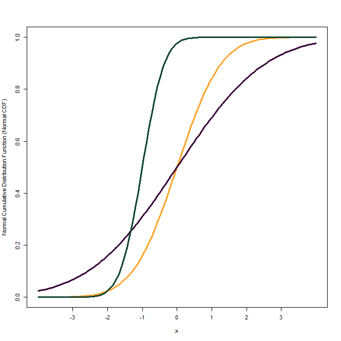
The first figure shows the Normal CDF of a Standard Normal Distribution which has a mean of 0 and standard deviation of 1. In the second figure, we have shown CDFs of Normal distributions with different means and standard deviations. The one in orange is the CDF of Standard Normal Distribution. The Normal CDF in dark green has a mean of -1 and a standard deviation of 0.5. Finally, the plot in dark purple has a mean of 0 same as the Standard Normal, but a higher standard deviation of 2.
This Normal CDF also has its applications in Statistics, Economics and Econometrics. For example, Normal CDF is used as a link function in the Probit Model with a qualitative dependent variable.
The Central Limit Theorem
The Central Limit Theorem (CLT), a cornerstone in probability theory, asserts that the sample means’ distribution transforms into a normal distribution with expanding sample sizes. This phenomenon of convergence is agnostic to the original distribution of the population and is contingent upon independent sample selection and a finite population variance, crucial for diverse statistical investigations in disciplines like economics and finance.
Essentially, the CLT posits that large, random samples from any population culminate in the sample means assuming a normal distribution, despite the variance in original population distributions. Its historical lineage traces back to early 19th-century rudimentary forms, evolving into a definitive structure by 1920, further amalgamating classical and modern probability theory. A critical tenet of the CLT elucidates how random fluctuations, surrounding a fixed parameter, trend towards a Gaussian distribution as the sample size increases.
The Empirical Rule in Normal Distribution
68-95-99.7 Rule
The empirical rule, known as the 68-95-99.7 rule, also aids in comprehending data spread in a normal distribution. It articulates that a significant portion of data falls within certain deviations from the mean: approximately 68.27% within one standard deviation, 95.45% within two, and 99.73% within three standard deviations. Moreover, its application extends to predictive analytics and thorough risk evaluation activities.
The 68-95-99.7 rule ensures, therefore, that a vast majority of the dataset is encapsulated within three standard deviations of the average. It significantly simplifies the determination of event probabilities and their associated likelihoods, bolstering its role in analytical scenarios.
Applications
Extensively employed in sectors reliant on meticulous risk assessment and foresight analytics, the rule is indispensable. In the field of finance, it also facilitates the assessment of market instability through the computation of standard deviations. For logistics, it is further instrumental in approximating delivery timelines. Its widespread application exemplifies its pivotal role in performing efficient data analysis.
While financial market data might not adhere strictly to a normal distribution, the use of standard deviation remains paramount in the estimation of financial risks and market fluctuations. Moreover, proficiency in applying these empirical principles equips professionals with the tools they need. This includes making data-informed decisions, maintaining quality surveillance, and forecasting results based on probabilistic evaluations.
Skewness in Normal Distribution
Skewness in a normal distribution signifies the extent of its asymmetry from the ideal bell curve symmetry. A normal distribution serves as a paramount case of symmetry, therefore, holding a skewness value of zero. This also implies equilibrium around its central mean.
Conversely, within distinct distributions, we also unearth disparate skewness characterizations. For example, the double exponential’s skewness registers around 0, stipulating symmetry whereas an exponential distribution has a skewness of 2.
Skewness wields critical implications in data analysis, especially within the economic and financial realms. A symmetric, zero-skewness normal distribution stands as a foundational model for economic prediction under complete symmetry. Real data items, however, typically manifest skewness, positive or negative, affecting a distribution’s tail lengths asymmetrically. This departure from ideal symmetry impacts financial prognosis and peril evaluation models, hence, necessitating skewness consideration within data scrutiny.
Kurtosis in Normal Distribution
Kurtosis delves into the distribution’s tail characteristics, offering insight into the data’s extremities and outliers. These characteristics include mesokurtic, platykurtic, and leptokurtic, each illuminating different data density profiles. Mesokurtic distributions, for example, mirror the normal curve with a kurtosis of approximately 3.
Leptokurtic distributions, with kurtosis above 3, signify an increased amount of outliers and thicker tails. Therefore, instances like the Student’s t-distribution highlight this phenomenon. Conversely, the term platykurtic describes distributions with kurtosis below 3, implying slender tails with fewer extreme values.
For investors, understanding kurtosis is pivotal to accurately gauge the risk in their investments, with high kurtosis further signalling a greater risk of extreme price movements. In the financial sector, professionals may rely on kurtosis for assessing the probability of these extreme events, also aiding in the formation of risk mitigation strategies. Analyzing a distribution’s kurtosis enables these experts to foresee the presence of fat tails accurately and make informed risk management decisions.
Examples of Normal Distribution
Grasping the manifestation of normal distribution in our day-to-day experiences also significantly enhances the linkage between theoretical and practical contexts. Hence, let us consider 2 examples of a normal distribution:
Height and Weight
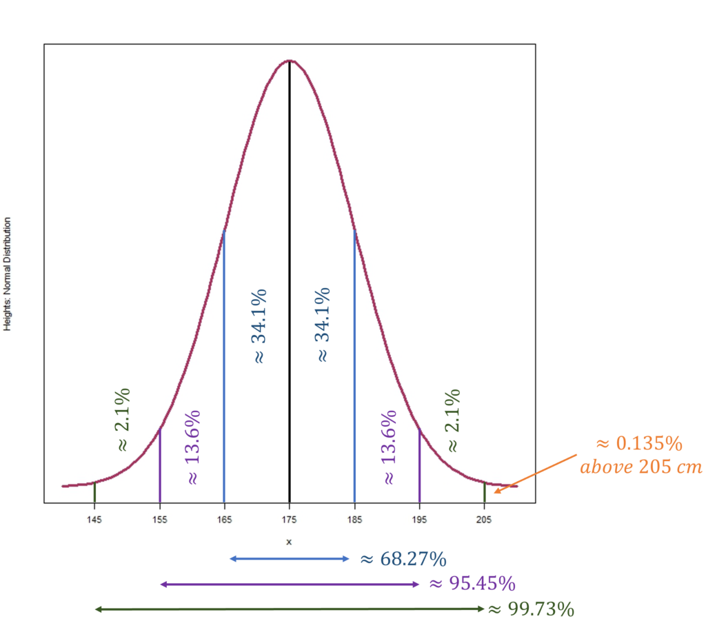
Classic examples of normal distribution include human height and weight variables. Suppose, the typical human height average approximates 175 cm. A normal distribution indicates that nearly 99.73% of individuals fall within three standard deviations from this average. For illustration, in a hypothetical town with adult heights conforming to a normal distribution, where the mean is 175 cm and the standard deviation is 10 cm, one would expect a minute fraction of the population, about 0.135%, to surpass 205 cm. If the town has a population of 330,000, this translates to roughly 446 individuals above 205 cm. Such insights further underscore the robustness and suitability of normal distribution in capturing the variances in human physical traits.
IQ Scores
Intelligence Quotient (IQ) scores represent another paramount domain for normal distribution analysis. Suppose, the standard IQ mean stands at 100, encapsulating a majority of the global intelligence metric. Approximately 68.27% of IQ scores encompass 1 standard deviation range from the mean, with 95.45% contained within a 2 standard deviations range, and nearly 99.73% lying within three deviations. The culminated distribution depicts a recognizable bell curve, hence, embodying the application of normal distribution in the understanding of human cognitive prowess.
Role of Normal Distribution in Economics
Asset Prices
The normal distribution also plays a central role in economic analysis, specifically in market evaluation and asset pricing appraisal. Through its utilization, economists can apply the bell curve to discern significant deviations in asset prices from the average. This method further unveils potential overvaluation or undervaluation scenarios, critical in investment decision-making.
Underpinning asset pricing mechanisms in financial markets is the supposition of returns conforming to a normal distribution. This paradigm simplifies return modelling and strategizing investments. Within a normal distribution, the majority of readings reside close to the mean, outlining a standard by which to evaluate asset value.
Market Analysis
Crucial to market analysis is the normal distribution, applied to project future market shifts and trends. However, it is imperative to acknowledge the inadequacy of this assumption alone, as real-world market returns often exhibit skewness and fat tails, signalling a departure from the norm. While foundational, reliance solely on the normal distribution proves insufficient. This further necessitates a blend of approaches and models to account for these irregularities in market dynamics and asset valuations.
Normal Distribution in Econometrics
Econometrics is also deeply grounded in the Gaussian distribution, essential for evaluating economic relationships and hypothesis testing. It operates under the assumption that regression model errors conform to a normal distribution, facilitating more precise economic parameter inferences and reliable future trend predictions. The Gaussian distribution’s symmetries and the empirical rule’s application cement its utility in econometric analyses.
Hence, the normal distribution is vital in econometrics for handling random variables in economic models. This simplification comes from the central limit theorem, which states that the average of large random samples with a finite mean and variance will tend to a normal distribution as the sample size increases. This theorem is foundational, also supporting a multitude of econometric methods and analyses.
Econometric techniques often employ normal distribution tables for probability calculations and inferences. These tables match Z-values with associated probabilities, further easing complex statistical work. The distribution’s unique features, like a symmetrical peak with the mean, median, and mode aligned, further enhance its utility and practicality in econometrics.
In assessing regression residuals, economists leverage the Gaussian distribution framework. If the residuals’ normality is confirmed, it verifies the model’s assumptions and the validity of the economic relationships under scrutiny. Hence, this step is pivotal in ensuring trustworthy and meaningful economic forecasts and policy decisions.
Normal Distribution in Other Fields
Economics and Econometrics are not the only fields where normal distribution is extensively employed. Normal distribution also forms the basis for hypothesis testing in clinical trials, an essential part of medicine and biostatistics. Moreover, in population studies, it is used to model attributes like height, weight, and blood pressure. This enables accurate forecasts of various demographic aspects.
Conclusion
Hence, the normal distribution is a fundamental aspect of statistical analysis and economic modelling. Its symmetrical, bell-shaped curve, characterized by mean and standard deviation, provides a powerful means for understanding and predicting data trends. Economists also rely on this distribution to model various economic phenomena, given its nature where the majority of observations cluster around the mean.
An essential feature of the normal distribution is its adherence to the 68-95-99.7 rule. This rule stipulates that a significant portion of data, around 68.27%, falls within one standard deviation of the mean. Moreover, 95.45% lie within two standard deviations, and an overwhelming 99.73% within three standard deviations. Such predictability simplifies decision-making processes for economists and data analysts in various fields.
Nonetheless, the utility of the normal distribution faces challenges, particularly in finance. Market prices’ fluctuation can lead to distributions with skewness and kurtosis beyond its capability. In light of these inaccuracies, there’s a requirement for economists and financial analysts to explore alternative modelling frameworks, to ensure a better fit for their datasets.
In summary, it serves as a critical backbone for economics and econometric modelling. Its foundational nature simplifies the interpretation of complex data, enhancing the clarity of economic theories and forecasts. Yet, due to its limitations, which are often glaring in the financial sector, a nuanced and cautious approach is crucial for its application in decision-making and analysis.
Econometrics Tutorials with Certificates

This website contains affiliate links. When you make a purchase through these links, we may earn a commission at no additional cost to you.