The Durbin-Wu-Hausman Test of Endogeneity is used to determine whether the endogenous regressors in a simultaneous equation model are truly endogenous. Simultaneous equation models include both endogenous and exogenous variables. The decision to take certain variables as endogenous generally depends on theoretical considerations or a priori information.
However, it is possible that the regressors treated as endogenous in the model may be exogenous in reality. Therefore, this test determines whether the regressors assumed to be endogenous in the model are truly endogenous or not. If the test indicates that those variables are exogenous, then a simultaneous equation model is not needed. Hence, we can estimate the given equations using Ordinary Least Squares (OLS) because they will give efficient and consistent results. If the regressors are truly endogenous, simultaneous equation models such as 2SLS should be used because OLS estimates will be biased and inconsistent.
Specification of Simultaneous equation model
Let us consider a simple simultaneous equation model for illustrating the use and interpretation of the Test of Endogeneity.
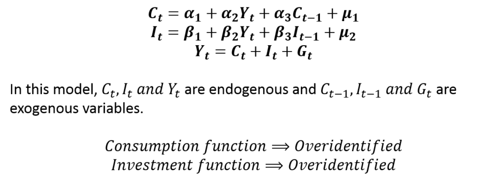
Since both the consumption and investment functions are overidentified, we can use Two-Stage Least Squares (2SLS) to estimate the equations.
Procedure of applying the test of endogeneity
In the above model, the consumption and investment equations have to be estimated one by one. This is because 2SLS is a single equation approach to simultaneous equation models. In our example, we will estimate only the consumption function/equation for illustration and apply the Test of Endogeneity to check whether Income (Yt) is truly endogenous.
Important: Test of Endogeneity is applied to endogenous regressors. That is, endogenous variables that appear on the right side of the equations. In this example, Income or Yt is the endogenous regressor. Hence, the Test of Endogeneity will determine whether Income (Yt) is truly endogenous or exogenous.
STEP 1:
Estimate the Reduced-Form equation of Yt (all exogenous variables included as independent and Yt as dependent variable). Therefore, we estimate the following equation:
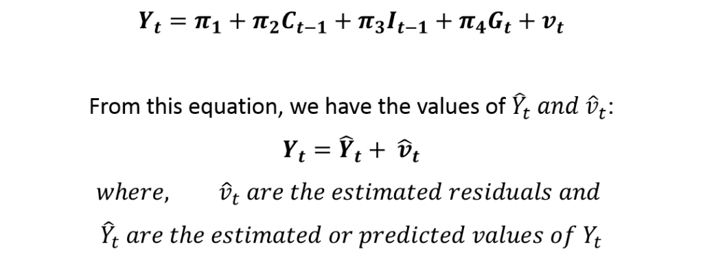
STEP 2:
We run a regression with Consumption (Ct)as the dependent variable and above “estimated residuals” (vt) as an independent variable along with other variables in the consumption function. Hence, we run the following regression:

The results of the above equation help us establish the Endogeneity or Exogeneity of Income (Yt).
STEP 3:
Test the following hypothesis:

Hence, if the above coefficient associated with estimated residuals (vt) is statistically significant, we conclude that the Income (Yt) variable is endogenous and apply the 2SLS model. If it is not significant, Yt is exogenous and we can simply use OLS to estimate the consumption function.
Application and interpretation in practice
In practice, the Test of Endogeneity will be applied after estimating the consumption function using the 2SLS approach. After obtaining the 2SLS estimates of the above consumption function, we applied the Test of Endogeneity. The results of the test are as follows:
| Test of Endogeneity | |
| H0: Yt is exogenous | |
| Durbin chi2(1) = 31.8962 | p = 0.0000 |
| Wu-Hausman F(1,58) = 61.4535 | p = 0.0000 |
The results of the test show that we can reject the null hypothesis because the p-value is less than 0.05. Hence, we can conclude that Yt is endogenous and the estimates of the 2SLS model are appropriate.
Before moving on to interpret the results of simultaneous equation models such as 2SLS, it is essential to apply this test of endogeneity. This is because the OLS estimates are efficient as well as consistent if the variables are exogenous. In presence of endogenous regressors, 2SLS estimates should be used because OLS estimates are inconsistent. The 2SLS estimates are biased but still consistent in the presence of endogenous regressors.
Econometrics Tutorials with Certificates
This website contains affiliate links. When you make a purchase through these links, we may earn a commission at no additional cost to you.

