The Vector Autoregression or VAR model is an essential tool in time series analysis. It is an extension of the univariate autoregressive models and can incorporate multiple time series variables, that is, the VAR model is a multivariate time series model. With its ability to analyze and forecast multivariate time series data, the VAR model provides valuable insights into the dynamic relationships between variables.
Vector autoregression (VAR) has a vast application in economics, finance and policy analysis. The VAR model is often used to examine the relationships between macroeconomic variables such as GDP, consumption, money supply and more.
Econometrics Tutorials with Certificates

Vector Autoregression or VAR Model Specification: Reduced-form VAR
The Vector Autoregression (VAR) Model can incorporate multiple time series variables. You can learn everything about the theory and application of the VAR Model from the VAR Model and IRFs tutorials. Suppose we have K variables in a VAR Model, then we can specify a basic Reduced-form VAR Model as shown here:
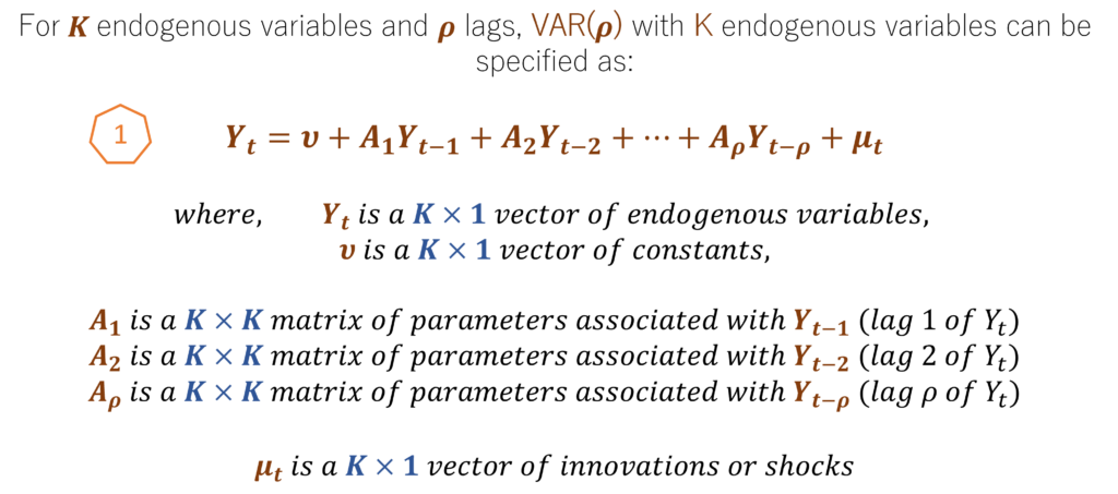
In a Reduced-form VAR like the one shown above, the endogenous variables in Yt depend only on their lags or past values. Therefore, none of the variables affect each other in the same time period and there are no contemporaneous effects. We can observe this on the right-hand side of the VAR model equation because the right side only has the lags Yt-1, Yt-2 and so on as explanatory variables.
The Yt ,Yt-1, Yt-2 and all the lags are K by 1 vectors of endogenous variables. For instance, if we have 3 endogenous variables in the VAR model, then they will be 3 by 1 vectors. The matrices A1, A2 and so on are coefficients matrices associated with the lags of the endogenous variables. These coefficient matrices will be K by K matrices. With K endogenous variables in the VAR model, we will have K number of equations and all the K equations are represented using this matrix representation of the VAR Model.
The ρ represents the number of lags of each endogenous variable in the VAR Model. For example if ρ = 4, then we will have 4 lags of endogenous variables included as the explanatory variables in every equation of the VAR Model. Appropriate lag-length selection is one of the most important steps in VAR estimation.
The innovations or residuals μt will further contain the reduced-form innovations of all the K equations of the VAR Model. These residuals are assumed to be white-noise and serially independent.
Extensions of the Reduced-form VAR Model
Exogenous variables and Deterministic terms
In the simple Reduced-form VAR Model specified earlier, we have not included any exogenous variables or deterministic terms except the constant or intercept. However, it is easy to incorporate deterministic terms like a trend or seasonal dummy variables. Many economic time series have a trend or exhibit seasonality. The Vector Autoregression or VAR Model can incorporate trends and include seasonal dummy variables within the equations to account for trending or seasonal behaviour. Most software programs provide an easy option to implement this and you can learn more about including these terms here.
Vector Error Correction Mechanism or VECM
The VECM Model is a special extension of the Reduced-form VAR Model used in situations of cointegration. Cointegration is a situation where the variables are non-stationary but their linear combination is stationary or has a lower order of integration. Such variables are said to have a common stochastic trend and a long-run relationship.
A basic Reduced-form VAR is not suitable in such situations and leads to misspecification because it cannot analyze both the short-run and long-run behaviour of the endogenous variables. Reduced-form VAR is generally applied to stationary variables. If the variables are non-stationary, we usually make them stationary by taking differences and giving us short-run estimates. However, if the variables are cointegrated, then a VAR in differences is not suitable because it ignores the long-run relationship among variables.
As a result, we consider the VECM Model if the variables cointegrated so we can incorporate short-run as well as long-run dynamics.
Structural VAR or SVAR
As mentioned earlier, Reduced-form VAR Models do not include contemporaneous effects. That is, the variables do not affect each other in the same time period. This approach is convenient but not always realistic. In reality, variables may affect each other instantly or without any time lag. In such a case, we can use Structural-VARs or SVARs instead of the Reduced-form VARs.
The SVAR models allow us to include contemporaneous effects and we can choose which variables can affect others instantly. Moreover, we can also introduce restrictions on the variables or structural shocks/innovations based on theoretical considerations or a-priori information. The Impulse Response Functions or IRFs are generally estimated using the structural shocks/innovations from the SVAR models.
In fact, the Reduced-form VAR coefficients and innovations are related to the SVAR coefficients and structural shocks. Therefore, we can derive the Reduced-form VAR from the SVAR Model. You can learn more about the relationship between the Reduced-form VAR and SVAR Models here.
Applications of the Vector Autoregression or VAR Model
We are usually not interested in interpreting the VAR coefficients. Instead, it is the further applications of the VAR Model that are most useful and these primarily include forecasting and impulse response functions (IRFs).
Forecasting
One of the most widely used post-estimation applications of VAR Models is dynamic forecasting. Forecasting is especially widespread in the case of macroeconomic variables and policy analysis. A feature of the Reduced-form VAR Model is that we can forecast the future using only the current and previous period values. Since we already have the current and previous period values, we can forecast the future for as many periods as we want.
In dynamic forecasting, we use the previous lags to forecast the current values of endogenous variables. Once we have the current forecasted values, we can use those forecasts to generate forecasts further into the future. Suppose we have a Reduced-form VAR model with 1 lag or VAR(1) model, then we only need the current period value (Yt) to forecast the next period (Yt+1). To forecast Yt+2, we can use the forecasted Yt+1. To forecast Yt+3, we can use the previous forecasted value Yt+2 and so on.
However, it is important to note that the forecasts will generally become less reliable as the forecast horizon increases. If we have exogenous variables in the VAR Model, then we will need data on the future time periods for the exogenous variables to generate the forecasts.
Impulse Response Functions (IRFs)
The Impulse Response Functions or IRFs analyze the effects of external shocks on the endogenous variables in the VAR, SVAR and VECM Models. IRFs are one of the most important applications of the VAR Models. Furthermore, we can estimate simple IRFs from the Reduced-form VAR Models or Orthogonolized IRFs from the Structural-VARs with contemporaneous effects.
Generally, we prefer to estimate OIRFs or Orthogonolized Impulse Response Functions because they incorporate contemporaneous effects. That is, variables and shocks can instantly affect the VAR system. As a result, these OIRFs are estimates using structural innovations and not Reduced-form VAR innovations. However, we can still estimate OIRFs after Reduced-form VAR because the SVAR shocks/innovations are related to the Reduced-from VAR innovations.
You can learn more about their relationship, derivation, estimation and application from the IRFs tutorials.
Conclusion
The vector autoregression or VAR Models have utility extending into various sectors and sub-fields of economics. VAR models have proven their worth in unravelling and forecasting complex issues including the prediction of economic trends.
In addition to the simple Reduced-form VAR Model, we also have more advanced extensions such as the SVAR and VECM Models. These extensions of the basic VAR model allow us to adapt the model to suit the researcher’s needs and analyze complex issues. The VAR models have been often observed to perform well in macroeconomic forecasting. Its VECM adaptation allows us to analyze long-run and short-run relationships among variables. The SVAR Model, on the other hand, allows us to include contemporaneous effects and is often used to analyze causal relationships among variables.
Vector Autoregression or VAR Model’s dynamic forecasting ability and its application in Impulse Response Functions make it an indispensable tool for econometric analysis.
Econometrics Tutorials with Certificates

This website contains affiliate links. When you make a purchase through these links, we may earn a commission at no additional cost to you.