Vector Error Correction Mechanism (VECM) models are a special application of VAR or Vector Autoregressive Models. The specification of VECM models involves the introduction of error correction terms into the VAR models. VECM methodology is used if the variables in the system have a long-run relationship, that is, they are cointegrated.
Moreover, every VAR model can be specified in the form of VECM by differencing the variables and introducing error correction terms. However, VECM is used only in the presence of cointegrating or long-run relationships. If there is no cointegration or if the variables are stationary, the VAR model should be applied. You can learn more about the interpretation of the VECM model in the VECM Estimation and Interpretation post.
Cointegration
Non-stationary variables are said to be cointegrated if their linear combination is stationary. For example, if two variables in a system are I(1) or integrated of order 1, but their linear regression yields an error term that is stationary. In such a case, we can say that the two variables are cointegrated and have a long-run relationship. Furthermore, such variables move together over time and share a common stochastic trend. You can learn more about it from the post on Cointegration: Meaning, Tests and Models.
The VECM model is, therefore, used to analyze cointegrated variables or cointegrating relationships. It provides a mechanism to understand the long-run as well as short-run behaviour of the variables in the system.
Vector Error Correction: Underlying VAR model
As stated earlier, every VAR model can be expressed in the form of VECM using differences and error correction terms. This also implies that every VECM model has an underlying VAR model. To understand the specification of VECM, we must look at the underlying VAR model specification.
Any VAR model can be specified in the matrix form as follows:

In VAR and VECM terminology, the error terms are referred to as impulses or innovations. To illustrate further, let us consider a VAR model with 2 variables and 3 lags:
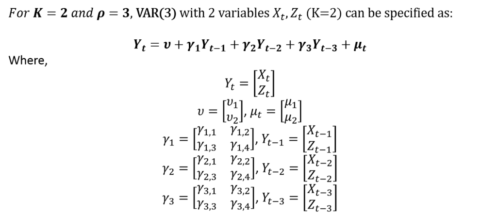
This VAR(3) with 2 variables (K = 2) is in the matrix form. Also, the appropriate lags (p) must be chosen with the help of Information Criteria. Moreover, the number of lags must ensure that there is no autocorrelation.
Cointegration and Vector Error Correction Mechanism (VECM)
The VECM models are specified in differences to account for short-run behaviour. Along with the short-run, VECM models also include error correction terms and cointegrating equations to account for short-run adjustments and long-run cointegrating relationships. Hence, the general form of a VECM can be specified as:
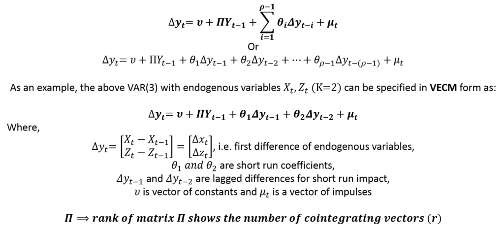
In the example, we can compare the VAR and VECM specifications for K = 2 model. The underlying VAR model has 3 lags, whereas, its VECM specification has 2 lags of differences. Therefore, the VECM form has one less lag (p – 1 lags) as compared to the underlying VAR model.
The Rank of the coefficient matrix associated with Yt-1 shows the number of cointegrating vectors (“r”). The number of cointegrating or long-run relationships (r) can be determined using Johansen’s Test of Cointegration.
Choosing between VAR and VECM
Tests of cointegration must be applied to ascertain whether the system of variables has any cointegrating relationships. Usually, Johansen’s Test of Cointegration is used to check for cointegration. Johansen provided a framework to check for cointegrating relationships and apply the Vector Error Correction Mechanism (VECM) to estimate short-run coefficients, short-run adjustment coefficients and long-run cointegrating relationships.
Using Johansen’s Test of Cointegration, we can determine “r”, which is the number of cointegrating vectors. In a system of “K” variables, there are 3 different scenarios:
| Number of cointegrating vectors (r) | Meaning | Stationarity of variables | Model to be used | Results |
| r = 0 | No cointegration | The variables are non-stationary and there are no long-run relationships among them | Apply VAR in differences | the VAR results show short-run coefficients |
| 0 < r < K | Cointegration exists | The variables are non-stationary and the number of cointegrating relationships is equal to “r” | Apply VECM | The VECM results show short-run coefficients and long-run equilibrium/cointegration relationship |
| r = K | No cointegration | The variables are stationary and cointegration cannot exist in stationary variables | Apply VAR to variables in their original form | The VAR results show long-run coefficients because the variables are not in differences |
Specification of VECM
Suppose, we determine that cointegration exists (0 < r < K) using Johansen’s Test of Cointegration. Then, we can specify the above VECM model as:
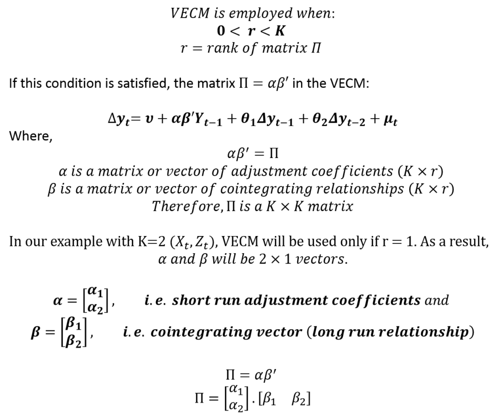
Hence, the VECM model gives us estimates of short-run behaviour, long-run cointegrating relationship as well as short-run adjustment coefficients. The short-run deviations from long-run equilibrium are corrected and the speed of this correction is shown by the adjustment coefficients.
The framework developed by Johansen allows the inclusion of several types of trends and constants in the short-run equations as well as in the cointegrating relationships. The specification of trends and constants differ according to the data. Some preliminary analysis is needed to determine the appropriate trend specifications. Let us consider all the trend specifications allowed under Johansen’s framework and when to employ them.
Specification of trends in VECM
Case 1: Unrestricted Trend
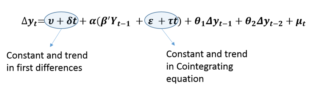
Firstly, an Unrestricted trend in a VECM means that we include a constant and a trend in the cointegrating equations as well as in the first differences. This specification implies a quadratic trend in the levels of variables because we are including a trend term in the first differences. Hence, this model should be used only if the variables show a quadratic trend. It is essential to plot the variables on a graph to check for quadratic trends or do formal testing for quadratic trends in the data.
The cointegrating equations are stationary around a time trend, that is, they are trend stationary. Hence, this specification allows the cointegrating equations to be trend stationary and original variables to have a quadratic trend.
Case 2: Restricted Trend
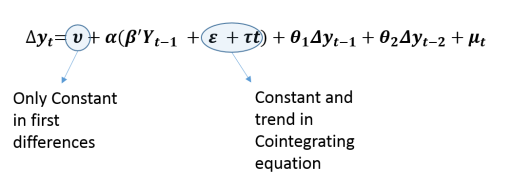
Secondly, Restricted trend specification does not include a trend in first differences, which implies a linear trend in original variables. In addition, it allows the cointegrating equations to be trend stationary. Hence, this specification should be used when the levels of variables have a linear trend and the cointegrating equations are stationary around a time trend, i.e. trend stationary.
In practice, a linear trend is easy to recognise. But, the trend stationarity of the cointegrating equations can be analyzed only after estimating the VECM. Therefore, it is advisable to estimate this model and then check whether a trend coefficient is needed in the cointegrating relationships or not.
Case 3: Unrestricted Constant
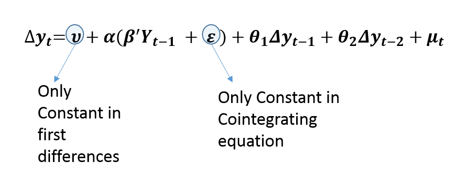
Thirdly, Unrestricted Constant is the most commonly used specification of VECM. Similar to the Restricted trend, it allows a linear trend in original or levels of variables. This is evident from the fact that we include only the constant term in the first differences. However, it is different from the Restricted trend specification because it includes only a constant in cointegrating relationships.
This specification allows the cointegrating or long-run relationship to be stationary around some constant mean. Hence, there is no trend in cointegrating relationships. As a result, it is used when there is a linear trend in original variables along with a cointegrating relationship that is stationary around some non-zero mean.
Case 4: Restricted Constant
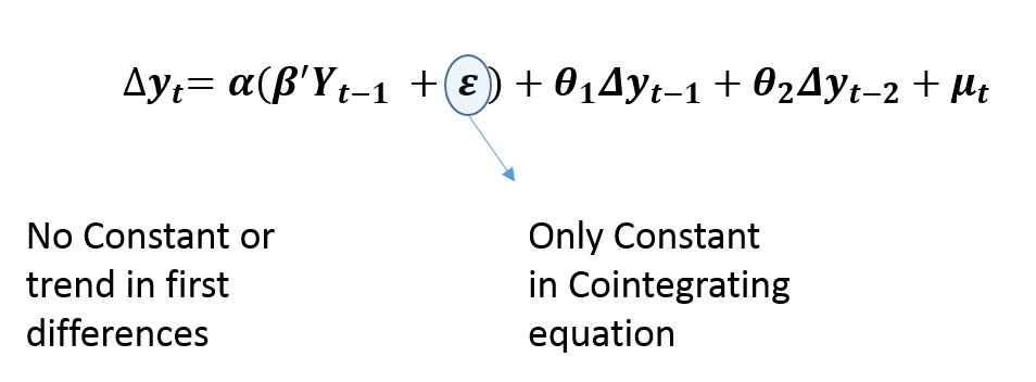
Restricted Constant specification does not include a constant or a trend in first differences. This implies that there is no trend in the levels of variables. It only allows a constant in the cointegrating relationships, meaning that it is stationary around a constant mean. This specification is used when the original variables do not show any linear trends and the cointegrating relationships are stationary around a constant mean without any trend.
Case 5: No Trend
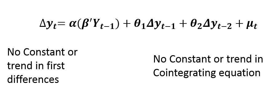
Finally, this specification of no trend is rarely used in practice. It does not include any trend or constant terms in the VECM model. It implies that the levels of variables show no trend and have zero means. Moreover, the cointegrating relationships are stationary around zero mean.
Econometrics Tutorials with Certificates


This website contains affiliate links. When you make a purchase through these links, we may earn a commission at no additional cost to you.
Good job, you simplified the topic. Look fwd to reading more of your blogs.
Thank you!!!!
Excellent analysis of the subject matter. U really demystified it.
Thank you!!!
Thank you, this is a very useful breakdown. Much appreciated.
You’re welcome